Session 1 Simple Regression
Chris Berry
2026
1.1 Overview
- Slides for the lecture accompanying this worksheet are on the DLE.
- R Studio online Access here using University log-in
In simple regression, we create a linear (straight line) model of the relationship between one outcome variable and one predictor variable
The outcome variable is what we want to predict or explain (e.g., anxiety scores)
The predictor variable is what we use to predict the outcome variable (e.g., average hours of screen time per week)
Both the outcome and predictor variable are continuous variables
Regression is actually a more general technique that underpins a wide variety of analyses. Simple regression is the most basic form of regression.
The simple regression equation has the form
Predicted outcome = a + b(Predictor)
a is the intercept, it is the height of the line. More formally, it's the value of the outcome when the predictor is equal to zero.
b is the slope (or coefficient for the predictor variable). It determines the steepness of the line, or, more formally, the amount of change in the outcome variable for a one unit increase in the predictor variable.
The goal of simple regression is to obtain the values of the intercept
(a) and slope (b) so that the line 'fits' or 'goes through' our data as
closely as possible. The specific method of 'fitting' the line to the
data is called the method of least squares (described in the lecture).
R can do this all automatically for us (with lm()).
1.2 Worked Example
Is screen time linked to mental health?
Teychenne and Hinkley (2016) used regression to investigate the association between anxiety and daily hours of screen time (e.g., TV, computer, or device use) in 528 mothers with young children.
Read in the data from their study to R and store in mentalh. The data
are located at
https://raw.githubusercontent.com/chrisjberry/Teaching/master/1_mental_health_data.csv.
Type or copy-paste the code to R Studio (e.g., in an Rmd file) to keep a record for your studies.
# ensure tidyverse is loaded
library(tidyverse)

# read the data to R using read_csv()
mentalh <- read_csv('https://raw.githubusercontent.com/chrisjberry/Teaching/master/1_mental_health_data.csv')
There are numerous variables in mentalh (use mentalh %>% glimpse()
to take a look). We will focus only on two here:
anxiety_score: a score representing the number of anxiety symptoms experienced in the past week, andscreen_time: hours per day of screen time use on average.
(Note: the data are publicly available with the article, but I've changed some of the variable names for clarity.)
First, create a scatterplot of the two variables. Put the predictor variable on the x-axis, and the outcome variable on the y-axis.
# The code below takes mentalh and pipes it to ggplot()
# aes() is used to tell ggplot() to put
# screen_time on the x-axis, and anxiety_score on the y-axis
# The settings in geom_smooth() tell ggplot() to
# add the regression line (method = 'lm') and
# not show confidence intervals (se = FALSE)

mentalh %>%
  ggplot(aes(x = screen_time, y = anxiety_score)) +
  geom_point() +
  geom_smooth(method = 'lm', se = FALSE)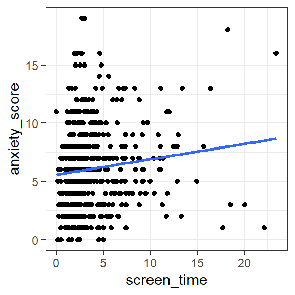
Figure 1.1: Scatterplot of anxiety score according to screen time (hours per day)
Exercise 1.1 Describe the relationship between screen time and anxiety evident in the scatterplot (pick one option; green = correct):
Use lm() to run the simple regression and store the results in
simple1:
# conduct a simple regression to predict anxiety_score from screen_time
# store the results in simple1
simple1 <- lm(anxiety_score ~ screen_time, data = mentalh)
Explanation: To specify the regression equation, we use
outcome_variable ~ predictor_variable.The ~ symbol is a tilde. We
use it to specify certain formulas in R. When you see ~, you can read
it as "as a function of". So, outcome variable ~ predictor variable
means "outcome variable as a function of the predictor variable". In our
case, "anxiety_score as a function of screen_time".
The intercept (a) and slope (b) are automatically calculated by R and
stored in simple1:
##
## Call:
## lm(formula = anxiety_score ~ screen_time, data = mentalh)
##
## Coefficients:
## (Intercept)  screen_time
##      5.5923       0.1318
Exercise 1.2
The value of the intercept a is
The value of the slope b for the screen_time predictor is
The regression equation Predicted Outcome = a + b(Predictor) can therefore be written as what?
1.3 Predicting
The regression equation can be used for prediction.
Suppose someone asked us what the anxiety_score would be for a new
person whose screen_time score is 10 hours per week.
By reading off from the regression line on the scatterplot from earlier,
the anxiety_score looks to be around 7:
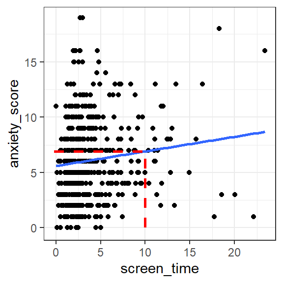
Figure 1.2: Predicted anxiety score for a person with 10 hours screen time
Using the regression equation, we can substitute 10 for screen_time,
then calculate predicted anxiety_score more precisely. The augment()
function in the broom package can be used to work out the prediction
for new data automatically:
# load the broom package
library(broom)

# store new scores as a tibble
new_scores <- tibble(screen_time = 10)

# give new_scores to 'newdata' option in augment()
augment(simple1, newdata = new_scores)| screen_time | .fitted |
|---|---|
| 10 | 6.91012 |
The predicted anxiety_score is in the .fitted column and is 6.91
Predictions for multiple individuals can also be made at once. Here we
obtain the predictions for two people with screen_time scores of 10
and 15.
# store the scores we want predictions for in new_scores
new_scores <- tibble(screen_time = c(10, 15))

# use augment() to obtain the predicted anxiety_scores
augment(simple1, newdata = new_scores)| screen_time | .fitted |
|---|---|
| 10 | 6.910120 |
| 15 | 7.569031 |
Each row shows one individual. Their predicted anxiety_scores are
6.91 and 7.57.
1.4 Residuals
The residual for a given datapoint is its vertical distance from the regression line. It is the error in prediction of the outcome variable for that datapoint.
Residual = Observed Score - Predicted Score
or
\(Residual = Y - \hat{Y}\)
where \(Y\) is the observed data point, and \(\hat{Y}\) is the predicted data point.
To view the residuals, again use the augment() function in the broom
package, this time without including newdata. The residual for each
observation is given in the column .resid
# look at the residuals for simple1 (in .resid)
# pipe to head() to only show the first 6 rows
augment(simple1) %>% head()| anxiety_score | screen_time | .fitted | .resid | .hat | .sigma | .cooksd | .std.resid |
|---|---|---|---|---|---|---|---|
| 7 | 2.571429 | 5.931167 | 1.068833 | 0.0022003 | 3.514985 | 0.0001024 | 0.304677 |
| 10 | 1.428571 | 5.780559 | 4.219441 | 0.0029659 | 3.510454 | 0.0021534 | 1.203238 |
| 13 | 4.214286 | 6.147666 | 6.852334 | 0.0019133 | 3.502526 | 0.0036559 | 1.953016 |
| 13 | 7.285714 | 6.552426 | 6.447574 | 0.0039508 | 3.503969 | 0.0067111 | 1.839532 |
| 3 | 18.571430 | 8.039682 | -5.039682 | 0.0402420 | 3.508118 | 0.0449817 | -1.464784 |
| 2 | 1.500000 | 5.789972 | -3.789972 | 0.0029045 | 3.511390 | 0.0017011 | -1.080735 |
Exercise 1.3 What was the residual for a person with anxiety_score equal to 13, and
screen_time score equal to 7.29?
For this person, was the anxiety score predicted by the model
The person has an anxiety_score of 13 and
screen_time score of 7.29. The predicted anxiety_score for this
datapoint is 6.55 (in the .fitted column), so the model underpredicts
the observed value of anxiety_score.
An assumption underlying regression is that the residuals are like random noise. More specifically, the residuals are assumed to be normally distributed with a mean of zero, and not correlated with one another.
When we plot the residual against the predicted values, there should also be no trend evident in the datapoints in the plot. We can use this plot for checking this assumption of regression.
# Create a plot of the predicted values vs. residuals
# Use the ".fitted" and ".resid" columns in augment()
# Use geom_hline() to draw a black horizontal line at y = 0
# Use geom_smooth() to fit a general trend line

augment(simple1) %>%
  ggplot(aes(x = .fitted, y = .resid)) +
  geom_point() +
  geom_hline(yintercept = 0) +
geom_smooth(color="blue", se=F) 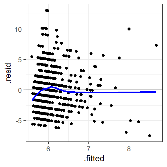
Figure 1.3: Predicted anxiety score vs. the residual
Explanation: If there's no trend in the residuals, we'd expect the
points to look like a random cloud above and below the horizontal line
(at y = 0). There should be no patterns, and the points should be pretty
symmetrically distributed around a single point in the middle of the
plot. There's some slight indication that the residuals tend to have
lower values as the predicted values (.fitted) increase. In other
words, there's some tendency for the model to overestimate
anxiety_score as screen_time becomes more extreme. The residuals
also seem more spread out above the horizontal at lower predicted
values, but this doesn't look too serious and the plot seems okay. The
blue line is the trend line drawn by RStudio, which also shows no
systematic trend. Issues here can indicate that improvement in the model
is possible.
Check the assumption that the residuals are normally distributed by obtaining a histogram:
# Create a histogram of the residuals using
# ggplot(aes())
# and geom_histogram()

augment(simple1) %>%
  ggplot(aes(.resid)) +
  geom_histogram()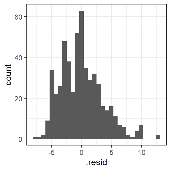
Figure 1.4: Histogram of the residuals
Explanation: Inspection of the histogram of residuals reveals that the distribution is approximately normal, satisfying this assumption.
1.5 Evaluating the model
1.5.1 R2
R2 is a statistic that describes how well our model explains the outcome variable. It ranges between 0 and 1 and can be interpreted as the proportion of variance in the outcome variable that is explained by the predictor variable.
To obtain R2 for the model:
| r.squared | adj.r.squared | sigma | statistic | p.value | df | logLik | AIC | BIC | deviance | df.residual | nobs |
|---|---|---|---|---|---|---|---|---|---|---|---|
| 0.0148346 | 0.0129617 | 3.511952 | 7.920493 | 0.0050709 | 1 | -1411.456 | 2828.913 | 2841.72 | 6487.581 | 526 | 528 |
The column r.squared contains R2 for the model, and is equal to
0.0148. To report as a percentage, multiply by 100. This means that
screen_time explains 1.48% of the variance in anxiety_score. In
psychological research, this is a relatively small amount of variance to
explain with a model. It may still be meaningful in some contexts though
(e.g., where it may be better to have a model with some predictive power
rather than none at all, or if a theory predicts a presence vs. absence of a relation).
In simple regression, R2 is actually the squared value of the Pearson correlation (r) between the outcome and predictor variable:
# load corrr package
library(corrr)

# obtain the Pearson correlation r between screen_time and anxiety_score
mentalh %>%
  select(screen_time, anxiety_score) %>%
correlate(method = "pearson")| term | screen_time | anxiety_score |
|---|---|---|
| screen_time | NA | 0.1217973 |
| anxiety_score | 0.1217973 | NA |
The correlation between screen_time and anxiety_score is r =
0.1217973.
0.1217973 * 0.1217973 = 0.0148, which is equal to the R2 value
obtained with glance()
1.5.2 Bayes factor
To further evaluate the model, we can obtain a Bayes factor (Rouder & Morey, 2012).
In simple regression, the Bayes factor tells us how much more likely the model is than one comprising the mean of the outcome variable only. We call this baseline model the intercept-only model. It is a model in which the regression line is a flat line (i.e., has a slope equal to zero), and the predictor does not predict the outcome at all.
To obtain the Bayes factor, use lmBF() in the BayesFactor
package:
# load BayesFactor package
library(BayesFactor)

# Compute the Bayes factor
lmBF(anxiety_score ~ screen_time, data = data.frame(mentalh))
## Bayes factor analysis
## --------------
## [1] screen_time : 4.465124 ±0%
##
## Against denominator:
## Intercept only
## ---
## Bayes factor type: BFlinearModel, JZSThe Bayes Factor is 4.47. We'd report this as BF10 = 4.47. This BF
means that a model consisting of screen_time alone as a predictor of
anxiety_score is over four times more likely than an intercept-only
model (in which screen_time has a zero-slope and so does not predict
anxiety_score). In other words, there's sufficient evidence to say
that screen_time predicts anxiety_score.
Reporting the simple regression in a report:
A simple regression was conducted to model the number of anxiety symptoms reported in the past week (anxiety score) from average hours of screen time usage per day (screen time). Screen time was found to have a positive association with anxiety scores, whereby individuals who reported greater levels of screen time also tended to have greater anxiety scores. The regression equation was "Predicted anxiety score = 5.59 + 0.13(screen time)", indicating that every hour of screen time use was associated with an increase in 0.13 in the anxiety score. Screen time explained only a small proportion of the variance in anxiety score, adjusted R2 value = 1.30%. The Bayes factor, comparing the model against an intercept-only model, was BF 10 = 4.47, indicating moderate evidence for the model, with it being over four times more likely than an intercept-only model.
1.6 Exercise
Exercise 1.4 Is screen time predicted by age?
In addition to screen time, Teychenne and Hinkley (2016) also asked
participants their age in years, recorded in age in the mentalh
dataset. Let's explore whether age predicts screen_time using simple
regression.
Adapt the code in this worksheet to do the following:
Try to do each one on your own first, before looking at the hint (or the solution).
1. Produce a scatterplot of age vs. screen_time
Pipe mentalh to ggplot() and use geom_point() and
geom_smooth(). Put the new predictor variable (age) on the x-axis and
the outcome variable (screen_time) on the y-axis.
Describe the relationship between age and screen time in the scatterplot (pick one):
2. Conduct a simple regression, with screen_time as the outcome
variable, and age as the predictor variable
Use lm() to specify the simple regression
What is the value of the intercept a (to two decimal places)?
What is the value of the slope b (to two decimal places)?
What is the regression equation?
Make sure you have stored the
regression results (e.g., in simple2), then use glance() with those
results
What proportion of variance in the screen time is explained by age? (Report the adjusted R-squared value, to two decimal places)
Report the value of adjusted R-squared as a percentage, to two decimal places: The adjusted R2 value is equal to %
Use
lmBF() to specify the model
How many times more likely is the model with age as a predictor of
screen_time, compared to an intercept-only model? (to two decimal
places)
5. Produce a plot of the fitted (predicted) values against the residuals
Use augment() with ggplot() and geom_point()
What type of trend is evident between the predicted values and the residuals?
No association is apparent, but the
points above the line appear to be more spread out than the points below
the horizontal line. This indicates that the model tends to
underestimate some of the screen time scores. This could be because the
screen time scores are positively skewed, e.g., see
mentalh %>% ggplot(aes(screen_time)) + geom_density(), and therefore
taking the log transform of the scores prior to analysis may improve
this plot (though may not necessarily change the outcome of the
analysis).
6. On balance, does age seem to be a good predictor of a person's daily screen time use?
Yes, the older the individuals were, the lower the screen time score tended to be. A model with age as a predictor of screen time explained only 1.68% of the variance in screen time scores (adjusted R2), but the Bayes factor (BF10 = 12.19) indicated strong evidence for this model compared to an intercept-only model. The regression equation was "Predicted screen time = 7.48 - 0.10(age)", indicating that an increase in age of one year was associated with a reduction of approximately 6 minutes (i.e., one tenth of 1 hour) of screen time per week.
1.7 Further Exercises
For those feeling confident with everything so far.
Exercise 1.5 Further Exercise
The variable physical_activity in the mentalh dataset is a measure
of moderate-to-vigorous physical activity, based on participant's self
reported weekly activity.
To what extent is participants' anxiety_score explained by their
physical_activity?
Investigate by producing the following:
- Scatterplot
- Correlation
- Simple regression model
- Adjusted R-squared value
- Bayes factor
On balance, does the anxiety_score seem to be predicted by
physical_activity?
# scatterplot
mentalh %>%
  ggplot(aes(x = physical_activity, y = anxiety_score)) +
  geom_point() +
  geom_smooth(method = 'lm', se = F) +
  xlab("Physical activity") +
  ylab("Anxiety score") +
  theme_classic()

# correlation
mentalh %>% select(anxiety_score, physical_activity) %>% correlate()

# simple regression model
model_activity <- lm(anxiety_score ~ physical_activity, data = mentalh)

# look at intercept and slope
model_activity

# look at plot of fitted values and residuals
augment(model_activity) %>%
  ggplot(aes(x=.fitted, y=.resid)) +
  geom_point() +
  geom_hline(yintercept = 0)

# look at R-squared
glance(model_activity)

# calculate Bayes Factor
lmBF(anxiety_score ~ physical_activity, data = mentalh)No, there's no evidence that the anxiety scores are predicted by self reported measures of moderate-to-vigorous levels of physical activity. The two measures showed virtually no correlation, r = -0.01. The regression equation was Predicted Anxiety Score = 6.23 - 0.0001(physical activity), and the model explained no variance in anxiety score with the adjusted R2 = -0.0017. The Bayes factor was equal to 0.10. Given that this value of the Bayes factor is less than 0.33, this indicates substantial evidence for the intercept-only model, compared to the simple regression model where physical activity is the sole predictor of anxiety scores. In other words, if we only had these two variables, the best predictor of anxiety scores would be the mean value of the anxiety scores.
Interestingly, although there appears to be no relationship between anxiety and physical activity in this sample of individuals (mothers), other populations do apparently show reductions in anxiety with greater levels of vigorous physical activity (e.g., in adolescents, see Hrafnkelsdottir et al., 2018).
1.8 Going further: p-values
An additional resource on using p-values in regression if you are curious (e.g., for your projects):
In keeping with our undergraduate curriculum, Bayes factors have been used as the main method of statistical inference here.
Frequentist methods of statistical inference, which rely on p-values, are still widely used in the psychological research literature, however.
To obtain the p-values for a simple regression, use summary(model_name). For the first simple regression in the worksheet:
##
## Call:
## lm(formula = anxiety_score ~ screen_time, data = mentalh)
##
## Residuals:
##     Min      1Q  Median      3Q     Max
## -7.5103 -2.7076 -0.1194  2.0782 13.0500
##
## Coefficients:
##             Estimate Std. Error t value Pr(>|t|)
## (Intercept)  5.59230    0.23757  23.540  < 2e-16 ***
## screen_time  0.13178    0.04683   2.814  0.00507 **
## ---
## Signif. codes:  0 '***' 0.001 '**' 0.01 '*' 0.05 '.' 0.1 ' ' 1
##
## Residual standard error: 3.512 on 526 degrees of freedom
## Multiple R-squared:  0.01483,    Adjusted R-squared:  0.01296
## F-statistic:  7.92 on 1 and 526 DF,  p-value: 0.005071
Explanation of the output:
Residuals: provides an indication of the discrepancy between the values of anxiety_score predicted by the model (i.e., the regression equation) and the actual values of anxiety_score. Roughly speaking, if the model does a good job in predicting anxiety_score, the residuals should be relatively small.
- The difference between
MinandMaxgives us some idea of the range of error in the prediction ofanxiety_Scoresscores. The difference in3Qand1Qis the interquartile range. Themedianof the residuals is -0.12.
Coefficients: contains tests of statistical significance for each of the coefficients. The values in the column headed Pr(>|t|) are the p-values associated with the t-values for the coefficients for each predictor. The t-values test a null hypothesis that the coefficients are equal to zero. A p-value less than .05 indicates that a predictor is statistically significant. More specifically, it is the probability of obtaining a t-statistic at least as extreme as the one observed, if the null hypothesis is true.
The row for the
(intercept)reports a t-test for whether the value of the intercept differs from zero. We're not usually interested in this test (so wouldn't report it).The row for
screen_timetests whether the value of its coefficient (0.13) differs from zero. A coefficient of zero would be expected if the predictor explained no variance in the outcome variable. The coefficient forentrex(0.13) is greater than zero in this case. We can report this by saying thatscreen_timeis a statistically significant predictor ofanxiety_score, b = 0.13, t(526) = 2.81, p < .01.
Multiple R-squared: This is \(R^2\), which, as before, is the proportion of variance in anxiety_score explained by screen_time. Here, \(R^2\) = 0.0148, or 1.48%.
Adjusted R-squared: Again, this is an estimate of \(R^2\), but adjusted for the population. Despite the usefulness of this statistic, most studies still tend to report only the (unadjusted) \(R^2\) value. If reporting the Adjusted R-squared value, be sure to label it clearly as such. Here, Adjusted R-squared = 0.013, or 1.30%.
F-statistic: This compares the variance in anxiety_score explained by the model with the variance that it does not explain (i.e., explained variance divided by unexplained variance). Higher values of F indicate that the model explains greater variance in an outcome variable. If the p-value associated with the F-statistic is less than .05, we can say that the model significantly predicts the outcome variable.
Hence, we can say that a model consisting of screen_time alone is a significant predictor of anxiety_score, F(1, 526) = 7.92, p < .01. Higher screen_time scores tend to be associated with higher anxiety_scores scores. If our model did not explain any variance in anxiety_score, we wouldn't expect this to be statistically significant.
- In simple regression, the null hypothesis being tested on the F-statistic is that the slope of the regression line in the population is equal to zero. You'll notice that this is actually equivalent to the t-test on the
screen_timecoefficient. So in simple regression, report the F-statistic for the overall regression or the t-test on the coefficient (not both). This equivalence between F and t does not hold true for multiple regression, as we shall see later.
The results of the frequentist and Bayesian analyses can be reported together in an article, e.g., "Hours of screen time significantly predicted anxiety score, b = 0.13, t(526) = 2.81, p < .01, BF10 = 4.47."
1.9 Summary
Simple regression can be used to model the relationship between an outcome and predictor variable, where both variables are continuous.
Once obtained, the regression equation allows us to:
precisely describe the relationship between the outcome and predictor variables (whether positive or negative).
derive predictions for the outcome variable, given new values of the predictor variable.
evaluate the model with R2 and use a Bayes factor to compare how much more likely it is to an intercept-only model.
Key functions
Visualise the data:
ggplot()Simple regression:
lm()R2:
glance()Residuals:
augment()Bayes Factor:
lmBF()
- In the next session we will explore regression models with more than one continuous predictor variable.
1.10 References
Hrafnkelsdottir S.M., Brychta R.J., Rognvaldsdottir V., Gestsdottir S., Chen K.Y., Johannsson E., et al. (2018) Less screen time and more frequent vigorous physical activity is associated with lower risk of reporting negative mental health symptoms among Icelandic adolescents. PLoS ONE 13(4): e0196286. https://doi.org/10.1371/journal.pone.0196286
Rouder, J. N., & Morey, R. D. (2012). Default Bayes factors for model selection in regression. Multivariate Behavioral Research, 47(6), 877-903. https://doi.org/10.1080/00273171.2012.734737
Teychenne M, & Hinkley T (2016) Associations between screen-based sedentary behaviour and anxiety symptoms in mothers with young children. PLoS ONE, 11(5): e0155696. https://doi.org/10.1371/journal.pone.0155696