Session 5 Multiple regression: hierarchical regression
Chris Berry
2026
5.1 Overview
- Slides for the lecture accompanying this worksheet are on the DLE.
- Slides for Rmd support are on the DLE.
- R Studio online Access here using University log-in
Hierarchical regression is another form of multiple regression analysis and can be used when we want to add predictor variables to a model in discrete steps or stages. The technique allows the unique contribution of the variables on each step to be separately determined.
We can use it when we want to know whether a predictor variable (e.g., sense_of_belonging) predicts an outcome (e.g., social_interaction) after controlling for background variables that are categorical (e.g., gender, level of education) or continuous (e.g., age, score on a cognitive test) in nature. The variables entered on each step can also be determined by theoretical considerations, to test specific hypotheses.
At each step in the analysis, the increase in the variance explained in the outcome variable (i.e., R2) and evidence for the unique contribution of the predictors (with Bayes factors) can be assessed.
Hierarchical regression is sometimes called sequential regression.
5.2 Worked example 1: wellbeing
In Session 2, we analysed some of the data from Iani et al. (2019) and found evidence that brooding and worry predicted wellbeing in a multiple regression.
Iani et al. (2019) were actually primarily interested in whether mindfulness and emotional intelligence predicted psychological wellbeing scores, but after controlling for brooding and worry. The reason for asking the question in this way is because it's a well-established finding that brooding and worry explain wellbeing, but less is known about mindfulness and emotional intelligence.
To control for brooding and worry, these variables are entered into a regression first. Next, mindfulness and emotional intelligence are added, and the change in R2 associated with their addition to the model can be evaluated. Bayes factors can also be used to assess the unique contribution of the predictors added at each step.
5.2.1 Read in the data
Read the data to R, and store in pwb_data (to stand for Psychological WellBeing data). The data we'll use are located at:
https://raw.githubusercontent.com/chrisjberry/Teaching/master/2_wellbeing_data.csv
# First ensure tidyverse is loaded, i.e., 'library(tidyverse)'

# read in the data using read_csv(), store in pwb_data
pwb_data <- read_csv('https://raw.githubusercontent.com/chrisjberry/Teaching/master/2_wellbeing_data.csv')(Note. The data are publicly available, but I've changed the variable names for clarity. As in Iani et al., missing values were replaced with the mean of the relevant variable.)
Preview the data with head():
| describing | observing | acting | nonreactivity | nonjudging | attention | clarity | repair | brooding | worry | wellbeing | gad |
|---|---|---|---|---|---|---|---|---|---|---|---|
| 13 | 14 | 19 | 6 | 15 | 23 | 20 | 21 | 18 | 19 | 64 | 13 |
| 15 | 6 | 15 | 13 | 12 | 24 | 20 | 15 | 14 | 30 | 72 | 7 |
| 14 | 14 | 16 | 17 | 11 | 31 | 27 | 26 | 15 | 30 | 59 | 11 |
| 10 | 10 | 18 | 18 | 18 | 27 | 18 | 20 | 16 | 29 | 62 | 13 |
| 10 | 14 | 15 | 14 | 16 | 21 | 24 | 14 | 8 | 27 | 78 | 5 |
| 21 | 15 | 18 | 14 | 14 | 30 | 26 | 23 | 10 | 23 | 78 | 4 |
About the data:
Mindfulness variables:
describing: Higher scores indicate greater ability to describe one's inner experiences.observing: Higher scores indicate greater levels of observing.acting: Higher scores indicate greater levels of acting with awareness.nonreactivity: Higher scores indicate greater levels of nonreactivity.nonjudging: Higher scores indicate greater levels of nonjudging.
Emotional intelligence variables:
attention: Higher scores indicate greater skill in attending to their feelings and moods.clarity: Higher scores indicate greater skill in experiencing their feelings clearly.repair: Higher scores indicate greater skill in regulating unpleasant moods or prolonging pleasant ones.
Negative functioning variables:
brooding: Higher scores indicate greater levels of brooding.worry: Higher scores indicate greater levels of worry.
Outcome variables:
wellbeing: Higher scores indicate higher levels of psychological wellbeing in terms of self-acceptance, positive relations with others, autonomy, environmental mastery, purpose in life, and personal growth.gad: higher scores indicate greater severity of Generalised Anxiety Disorder.
5.2.2 Visualisation
There are a number of continuous variables in the dataset that we can visualise with density plots or histograms. We've done this individually, variable by variable in past worksheets. Here I'd like to show you a more advanced way of plotting. The code below will create a density plot of every variable in a dataset that is numeric (continuous) in nature, using different facets:
# Plot density plots of all the numeric (continuous) variables
# The code below:
# -Keeps only the numeric columns in a data frame
# -Uses pivot_longer() to code each set of scores by its variable name
# -Specifies the 'score' to plot in aes()
# -Uses facet_wrap() to plot each variable in a separate panel
# -Uses scales = "free" to allow the range on the x- and y-axis to be different across panels

pwb_data %>%
  keep(is.numeric) %>%
  pivot_longer(everything(), names_to = "variable", values_to = "score") %>%
  ggplot(aes(score)) +
  facet_wrap(~ variable, scales = "free") +
geom_density() 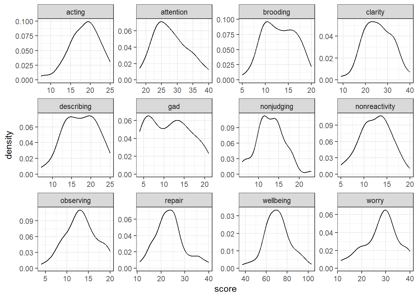
Figure 2.1: Density plots for each continous predictor in pwb_data
5.2.3 Correlations
With many variables being used in a multiple regression, it is good practice to inspect the correlations between all continuous variables first to get an idea of the inter-relations and to check for multicollinearity between predictors.
Obtain a correlation matrix of all of the numeric variables. Ensure the corrr package is loaded, then use correlate():
# library(corrr) # ensure this is loaded

# correlations of all numeric variables
# use mutate() with round() to round to 2 D.P.
pwb_data %>%
  keep(is.numeric) %>%
  correlate(method = "pearson") %>%
  mutate(across(where(is.numeric), round, digits = 2))
Exercise 5.1 Before conducting the hierarchical regression, Iani et al. (2019) reported the Pearson correlations between wellbeing and gad and the mindfulness and emotional intelligence variables. We'll report a subset of those here to check you can read the correlation matrix that's output. Report the correlations below to two decimal places:
describingandclarity, r =describingandwellbeing, r =repairandwellbeing, r =nonreactivityandbrooding, r =nonreactivityandgad, r =
- Does multicollinearity seem an issue (check the correlations between the predictor variables for r < -0.8 or r > 0.8)?
5.2.4 Hierarchical regression
To conduct the hierarchical regression, variables will be entered to the multiple regression in progressive steps, and the change in R2 associated with the predictors added to the model at each step obtained. Likewise, Bayes factors can be used to determine whether there is evidence that the predictors added at each step make a unique contribution to the prediction of the outcome variable.
Iani et al. (2019) wanted to explain variance in wellbeing (the outcome variable). They reported the non-adjusted R2, so that's what we'll do too. Due to theoretical considerations, the variables in each step were entered as follows:
- Step 1:
brooding - Step 2:
brooding,worry - Step 3:
brooding,worryand mindfulness variables (describing,observing,acting,nonreactivity,nonjudging) - Step 4:
brooding,worry, mindfulness variables (describing,observing,acting,nonreactivity,nonjudging), and emotional intelligence variables (attention,clarity,repair).
5.2.4.1 Step 1: brooding
First, use brooding to predict wellbeing. Use lm() and glance() to obtain the R2 for the model, then use lmBF() to obtain the BF for the model.
# specify the model in the step
step1 <- lm(wellbeing ~ brooding, data = pwb_data)

# R^2^
# ensure the broom package loaded, i.e., with 'library(broom)'
glance(step1)

# store the BF
# ensure the BayesFactor package is loaded, i.e., with 'library(BayesFactor)
BF_step1 <- lmBF(wellbeing ~ brooding, data = data.frame(pwb_data))

# look at BF
BF_step1| r.squared | adj.r.squared | sigma | statistic | p.value | df | logLik | AIC | BIC | deviance | df.residual | nobs |
|---|---|---|---|---|---|---|---|---|---|---|---|
| 0.189052 | 0.1763809 | 11.4776 | 14.91998 | 0.0002642 | 1 | -253.7007 | 513.4014 | 519.9704 | 8431.064 | 64 | 66 |
## Bayes factor analysis
## --------------
## [1] brooding : 95.76111 ±0%
##
## Against denominator:
##   Intercept only
## ---
## Bayes factor type: BFlinearModel, JZS- The R2 (non-adjusted, as a proportion, to 2 decimal places) for the model in Step 1 = .
- The BF for the model in Step 1 =
5.2.4.2 Step 2: brooding + worry
Next, add worry to the model in Step 1, using + worry and look at R2 again and obtain the BF. We'll look at:
- whether the model in Step 2 explains more variance in
wellbeingby looking at the amount that R2 increases. - whether there's evidence for a contribution of
worryafter controlling forbrooding, by dividing the Bayes factor for the model in Step 2 by the BF for the model in Step 1
# specify the model in the step
step2 <- lm(wellbeing ~ brooding + worry, data = pwb_data)

# R-sq
glance(step2)

# store the BF
BF_step2 <- lmBF(wellbeing ~ brooding + worry, data = data.frame(pwb_data))

# compare the BFs for the models in Step 2 and Step 1
BF_step2 / BF_step1| r.squared | adj.r.squared | sigma | statistic | p.value | df | logLik | AIC | BIC | deviance | df.residual | nobs |
|---|---|---|---|---|---|---|---|---|---|---|---|
| 0.3288693 | 0.3075636 | 10.52393 | 15.43572 | 3.5e-06 | 2 | -247.4558 | 502.9116 | 511.6702 | 6977.446 | 63 | 66 |
## Bayes factor analysis
## --------------
## [1] brooding + worry : 56.11175 ±0%
##
## Against denominator:
##   wellbeing ~ brooding
## ---
## Bayes factor type: BFlinearModel, JZS- The R2 for the model in Step 2 is
- The increase in R2 associated with the addition of
worryto the model is Hint. To calculate this, take the R2 that you recorded before for the model in Step 2 and subtract the R2 for the model in Step 1. - The BF for the contribution of
worryto the model is . Hint. This is the BF produced by dividing the BF for the model in Step 2, by the BF for the model in Step 1.
Did you know that R can function like a calculator too? Simply type the formula next to > in the console window and hit enter, e.g., > 2 + 2
Or use code in your script:
In reports and articles, you will often see the change in R2 written as \(\Delta R^2\). The \(\Delta\) symbol means "change". For example \(\Delta R^2 = 0.33\).
5.2.4.3 Step 3: brooding + worry + mindfulness variables
Next, add the variables associated with mindfulness to the model. The mindfulness measures are observing, describing, acting, nonjudging, and nonreactivity. Add these five variables to the model all in the same step. As before, note R2 for the model and the BF. To determine whether there's evidence for the addition of the mindfulness variables, compare the BF for the model in Step 3 and the BF of the model in Step 2.
# specify the model in the step
step3 <- lm(wellbeing ~ brooding + worry +
             observing + describing + acting + nonjudging + nonreactivity,
            data = pwb_data)

# R-sq
glance(step3)

# store the BF
BF_step3 <- lmBF(wellbeing ~ brooding + worry +
                   observing + describing + acting + nonjudging + nonreactivity,
                 data = data.frame(pwb_data))

# compare the BFs for the models in step 3 and step 2
BF_step3 / BF_step2| r.squared | adj.r.squared | sigma | statistic | p.value | df | logLik | AIC | BIC | deviance | df.residual | nobs |
|---|---|---|---|---|---|---|---|---|---|---|---|
| 0.5330601 | 0.4767053 | 9.148738 | 9.458999 | 1e-07 | 7 | -235.4846 | 488.9692 | 508.6761 | 4854.566 | 58 | 66 |
## Bayes factor analysis
## --------------
## [1] brooding + worry + observing + describing + acting + nonjudging + nonreactivity : 35.49308 ±0%
##
## Against denominator:
##   wellbeing ~ brooding + worry
## ---
## Bayes factor type: BFlinearModel, JZS- The R2 for the model in Step 3 is
- The increase in R2 associated with the addition of the mindfulness variables is Hint. Take the R2 for the model in Step 3 and subtract the R2 for the model in Step 2.
- The BF for the contribution of the mindfulness variables to the model is Hint. This is the BF produced by dividing
BF_step3byBF_step2. - After controlling for
broodingandworry, is there sufficient evidence for the contribution of mindfulness to the prediction ofwellbeing?
The BF comparing the models in Steps 3 and 2 was BF = 34.59, indicating that the model in Step 3 is more than thirty five times more likely than the model in Step 2, given the data. Thus, there's substantial evidence that the mindfulness variables contribute to the prediction of wellbeing after controlling for brooding and worry. The mindfulness variables explain an additional R2 = 0.20, or 20% of the variance in wellbeing, over and above brooding and worry.
5.2.4.4 Step 4: brooding + worry + mindfulness + emotional intelligence variables
Next, add the variables associated with emotional intelligence to the model. The emotional intelligence variables are attention, clarity, and repair. These three variables are added to the model all in the same step. Once again, note R2 for the model and the BF. To determine whether there's evidence for the addition of the emotional intelligence variables, compare the BF for the model in Step 4 and the BF of the model in Step 3.
# specify the model in step 4
step4 <- lm(wellbeing ~ brooding + worry +
              observing + describing + acting + nonjudging + nonreactivity +
              attention + clarity + repair,
            data = pwb_data)

# R-sq
glance(step4)

# store the BF
BF_step4 <- lmBF(wellbeing ~ brooding + worry +
                   observing + describing + acting + nonjudging + nonreactivity +
                   attention + clarity + repair,
                 data = data.frame(pwb_data))

# compare the BFs for the models in step 4 and step 3
BF_step4 / BF_step3| r.squared | adj.r.squared | sigma | statistic | p.value | df | logLik | AIC | BIC | deviance | df.residual | nobs |
|---|---|---|---|---|---|---|---|---|---|---|---|
| 0.6045859 | 0.5326924 | 8.645487 | 8.409467 | 0 | 10 | -229.9978 | 483.9956 | 510.2715 | 4110.944 | 55 | 66 |
## Bayes factor analysis
## --------------
## [1] brooding + worry + observing + describing + acting + nonjudging + nonreactivity + attention + clarity + repair : 2.150042 ±0%
##
## Against denominator:
##   wellbeing ~ brooding + worry + observing + describing + acting + nonjudging + nonreactivity
## ---
## Bayes factor type: BFlinearModel, JZS- The R2 for the model in Step 4 is
- The increase in R2 associated with the addition of the emotional intelligence variables is Hint. Take the R2 for the model in Step 4 and subtract the R2 for the model in Step 3.
- The BF representing the evidence for the unique contribution of the emotional intelligence variables to the model is
- After controlling for
brooding,worry, and mindfulness, is there sufficient evidence for the contribution of emotional intelligence to the prediction ofwellbeing?
The BF comparing the models in steps 4 and 3 was BF = 2.15. Although this indicates that the model in Step 4 is more than twice as likely than the model in Step 3, given the data, the BF is less than 3, and therefore falls short of the conventional level for declaring that there's substantial evidence for the addition of emotional intelligence. Thus, according to this Bayes factor analysis, there's insufficient evidence that the additional R2 = 0.07, or 7%, of the variance in wellbeing explained by emotional intelligence represents a genuine improvement in prediction.
5.3 Exercise 1
Exercise 5.2 Hierarchical regression
Iani et al. (2019) were also interested in whether whether mindfulness and emotional intelligence predicted gad (anxiety symptoms) after controlling for brooding and worry.
Repeat the analysis conducted above, but now with gad as the outcome variable.
- Step 1:
brooding - Step 2:
brooding,worry - Step 3:
brooding,worryand mindfulness variables (describing,observing,acting,nonreactivity,nonjudging) - Step 4:
brooding,worry, mindfulness variables (describing,observing,acting,nonreactivity,nonjudging), and emotional intelligence variables (attention,clarity,repair).
Step 1: brooding
- The R2 (non-adjusted, to two decimal places) for the model in Step 1 =
- The BF for the model in Step 1 =
Rounding can sometimes be unclear when the last digit ends in a 5, and you are unsure of the precision to which something has been printed in the output R gives.
If in doubt, it's better to round from the more precise value. For R2, this can be obtained as follows from the glance function:
Step 2: brooding + worry
- The R2 for the model in Step 2 is
- The increase in R2 associated with the addition of
worryis - The BF for the contribution of
worryto the model is
Next, add worry to the model, using + worry. Look at R2 again and obtain the BF.
- To determine the R2 change for the model, take the R2 for the model in Step 2 and subtract the R2 value for the model in Step 1.
- To determine whether there's evidence for a contribution of
worryafter controlling forbrooding, divide the Bayes factor for the model by the BF for the model in Step 1.
Step 3: brooding + worry + mindfulness variables
- The R2 for the model in Step 3 is
- The increase in R2 associated with the addition of the mindfulness variables is
- The BF for the contribution of the mindfulness variables to the model is
- After controlling for
broodingandworry, is there sufficient evidence for the contribution of mindfulness to the prediction ofgad? - There's evidence for the model in Step 2, compared to Step 3, because the Bayes factor for the model in Step 3 divided by that of the model in Step 2 is .
Add the variables associated with mindfulness to the model. The mindfulness measures are observing, describing, acting, nonjudging, and nonreactivity. These five variables are added to the model all in the same step.
- To calculate the increase in R2, take the R2 for the model in Step 3 and subtract the R2 for the model in Step 2.
- To obtain the BF for the contribution of the mindfulness variables, take the BF for the model in Step 3 and divide it by the BF for the model in Step 2.
- If the BF is greater than 3, there's substantial evidence for the model in Step 3. If the BF < 0.33, then there's substantial evidence for the model in Step 2. Intermediate BFs are inconclusive.
# specify the model in Step 3
gad3 <- lm(gad ~ brooding + worry +
              observing + describing + acting +
              nonjudging + nonreactivity,
            data = pwb_data)

# R-sq
glance(gad3)

# store the BF
BF_gad3 <- lmBF(gad ~ brooding + worry +
                   observing + describing + acting +
                   nonjudging + nonreactivity,
                 data = data.frame(pwb_data))

# compare the BFs for the models in Step 3 and Step 2
BF_gad3 / BF_gad2
Step 4: brooding + worry + mindfulness + emotional intelligence variables
- The R2 for the model in Step 4 is
- The increase in R2 associated with the addition of the emotional intelligence variables to the model is .
- The BF associated with the contribution of the emotional intelligence variables to the model is
- After controlling for
brooding,worry, and mindfulness, is there sufficient evidence for the contribution of emotional intelligence to the prediction ofgad?
Add the variables associated with emotional intelligence to the model. The emotional intelligence measures are attention, clarity, and repair. These three variables are added to the model all in the same step.
- To calculate the increase in R2, take the R2 for the model in Step 4 and subtract the R2 for the model in Step 3.
- To obtain the BF for the contribution of the emotional intelligence variables, take the BF for the model in Step 4 and divide it by the BF for the model in Step 3.
- If the BF is greater than 3, there's substantial evidence for the model in Step 4. If the BF < 0.33, then there's substantial evidence for the model in Step 3. Intermediate BFs are inconclusive.
# specify the model in Step 4
gad4 <- lm(gad ~ brooding + worry +
                  observing + describing + acting + nonjudging + nonreactivity +
                  attention + clarity + repair,
                  data = pwb_data)

# R-sq
glance(gad4)

# store the BF
BF_gad4 <- lmBF(gad ~ brooding + worry +
                       observing + describing + acting + nonjudging + nonreactivity +
                       attention + clarity + repair,
                       data = data.frame(pwb_data))

# compare the BFs for the models in Step 3 and Step 2
BF_gad4 / BF_gad3
In summary, regarding the hypothesis of Iani et al. (2019):
- After controlling for
broodingandworry, there's evidence for the contribution of mindfulness and emotional intelligence to the prediction ofgad.
5.4 Worked Exercise 2: Controlling for categorical variables
All of the variables considered in the previous exercise were continuous (or at were least assumed to be). It is also possible to use hierarchical regression to control for the influence of variables that are categorical in nature.
How do human-animal relationships affect mental health? Ratschen et al. (2020) looked at the impact of relationships with animals (e.g., pets) on mental health and loneliness in individuals during the Covid-19 pandemic.
Data from their study are located at the link below.
https://raw.githubusercontent.com/chrisjberry/Teaching/master/5_animal_data.csv
The data are publicly available and variable names have been changed here for clarity. Missing data have been dealt with differently to the way the researchers dealt with them, so the data you are analysing (and therefore the results) are not identical to theirs.
About the data:
comfort: Comfort from companion animals. Higher scores indicate greater comfort from the companion animal.mental_health_pre: Mental health before lockdown. Higher scores indicate better mental health.mental_health_since: Mental health during lockdown. Higher scores indicate better mental health.wellbeing_since: Higher scores indicate better wellbeing.gender: Male, female, another option, or prefer not to sayage: Age group.partner: Whether the participant lives with their partner or not.species: The type of animal companion.loneliness_pre: Loneliness before lockdown. Higher scores indicate greater loneliness.loneliness_since: Loneliness during lockdown. Higher scores indicate greater loneliness.
5.4.1 Visualisation
Inspect the distributions of the continuous variables:
# Read in the data
animal_data <-
  read_csv('https://raw.githubusercontent.com/chrisjberry/Teaching/master/5_animal_data.csv')


# Plot density plots of all the numeric (continuous) variables
# The code below:
# -Keeps only the numeric columns in a data frame
# -Uses pivot_longer() to code each set of scores by its variable name
# -Specifies the 'score' to plot in aes()
# -Uses facet_wrap() to plot each variable in a separate panel
# -Uses scales = "free" to allow the range on the x- and y-axis to be different across panels

animal_data %>%
  keep(is.numeric) %>%
  pivot_longer(everything(), names_to = "variable", values_to = "score") %>%
  ggplot(aes(score)) +
  facet_wrap(~ variable, scales = "free") +
geom_histogram() 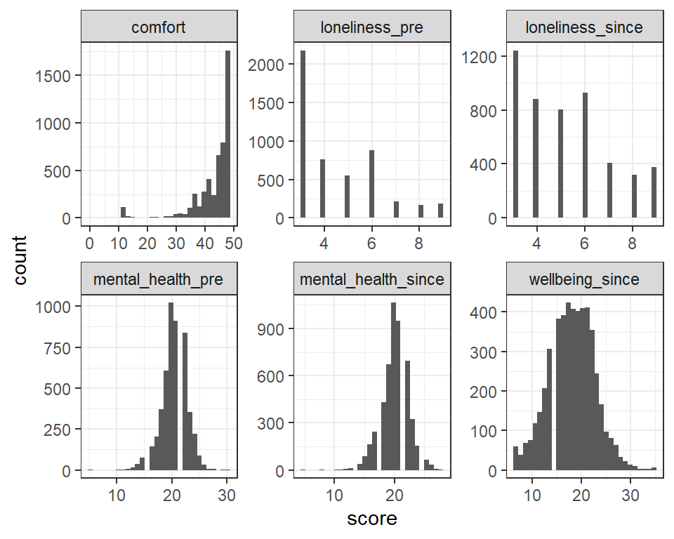
Figure 5.1: Histogram plots for each continous predictor
The code can be modified to obtain histograms of all of the categorical variables:
# Plot histograms of all the categorical vars (i.e. count data)
# The code:
# -Keeps only the character columns in the dataset
# -Uses pivot_longer() to code each set of scores by variable
# -Specifies the 'score' to plot in aes()
# -Uses facet_wrap() to plot in separate panels
# -Tells geom_histogram() to plot count data

animal_data %>%
  keep(is.character)  %>%
  pivot_longer(everything(), names_to = "variable", values_to = "score") %>%
  ggplot(aes(score)) +
  facet_wrap(~ variable, scales = "free") +
geom_histogram(stat = "count") 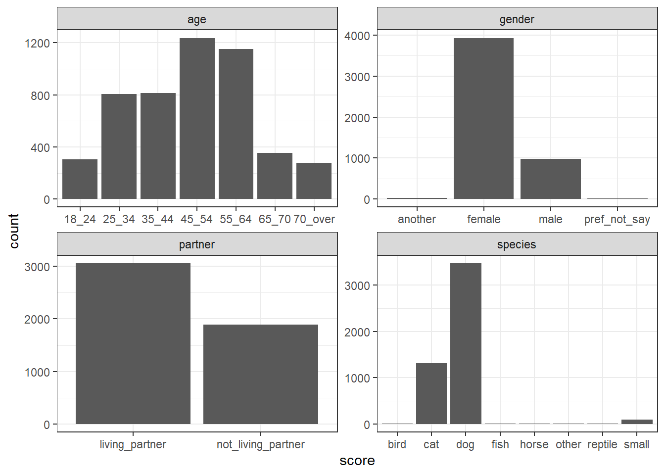
Figure 5.2: Histograms for each categorical predictor
By looking at the histograms of the categorical variables, answer the following:
- Age: The majority of people were in age group
- Gender: The majority of people were
- Partner: The majority of people were
- Species: The most common animal companion was
The scores on the loneliness_pre variable range from 3 to 9, so there are only 7 possible scores. When there are many data points, this can create issues when visualising the variable in a scatterplot because there are only so many combinations of scores for the variable, so they overlap.
The code below uses the gridExtra package to display two plots created with ggplot(). Each plot is stored in a separate variable panel1 and panel2, then placed side-by-side using grid.arrange() from the gridExtra package:
# load library(gridExtra)
# for displaying different plots on multiple panels
library(gridExtra)

# create a scatterplot of loneliness scores
# without random jittering of points
# store in panel1
panel1 <-
  animal_data %>%
    ggplot(aes(x=loneliness_pre, y = loneliness_since)) +
    geom_point() +
    geom_smooth(method="lm", se = F) +
    ggtitle("Without geom_jitter()")

# create a scatterplot of loneliness scores
# with random jittering of points using geom_jitter()
# store in panel2
panel2 <-
  animal_data %>%
    ggplot(aes(x=loneliness_pre, y = loneliness_since)) +
    geom_jitter() +
    geom_smooth(method="lm", se = F)+
    ggtitle("With geom_jitter()")

grid.arrange(panel1, panel2, nrow = 1)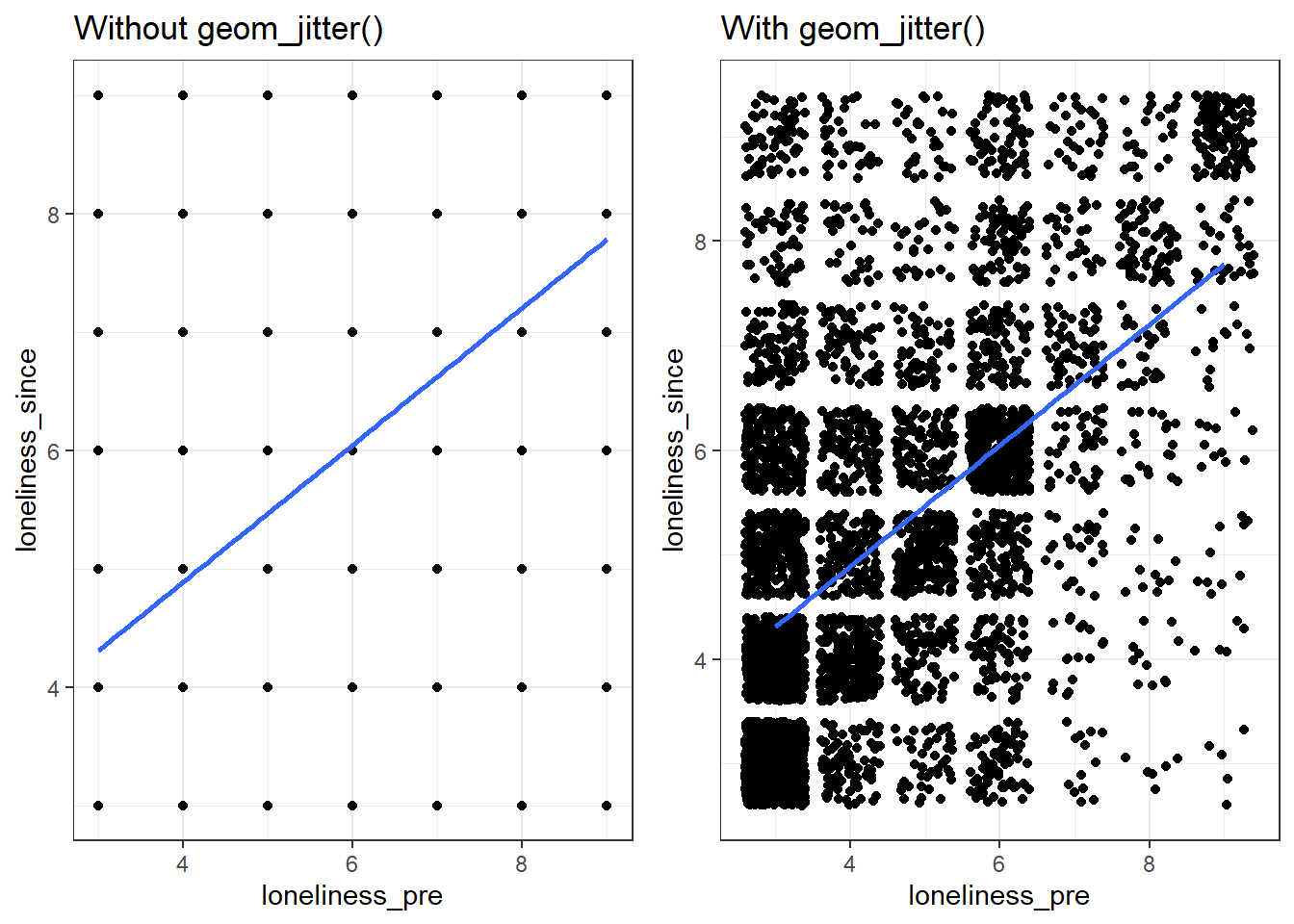
Figure 2.3: Using geom_jitter(): loneliness_since vs. londliness_pre
Using geom_jitter() instead of geom_point() means that the scores will be randomly jittered by a tiny amount. This reduces overlap, making it much easier to see how the scores are distributed. It's useful to use geom_jitter() when the response variable is on an ordinal scale, but the responses are discrete (e.g., 1, 2, 3, 4, 5), as is often the case with survey data and likert scales. Thus, if you ever create a scatterplot of survey data and it ends up looking like the plot on the left, try using geom_jitter() instead of geom_point().
The next step isn't strictly necessary because the categorical variables are stored as character variables (i.e., <chr>), but it is good practice to convert the categorical variables to factors before the analysis.
5.5 Exercise 2
Exercise 5.3 Hierarchical regression
Using the animal_data, we'll look at whether comfort scores predict mental_health_pre after controlling for gender, age, partner, species and loneliness_pre.
- How many steps do you think there'll be in the hierarchical regression analyses?
The variables we want to control for can go into the model in the Step 1. Then we can add comfort to the model in Step 2, to see whether it explains mental_health_pre over and above all the variables in Step 1.
- How many participants are in this dataset?
The number of participants is the same as the number of rows. One way of checking is as follows:
The variables that are controlled for in a multiple regression are sometimes called covariates
Step 1: Covariates only
- R2 for the model containing the covariates only is (to three decimal places; this level of precision is required for this answer)
- The BF for the model containing the covariates only is
Run a regression to predict mental_health_pre from the covariates only. The covariates are the things we want to control for, and are gender, age, partner, species and loneliness_pre.
- Obtain R2 for the model using
glance()in thebroompackage. - Obtain the BF for the model using
lmBF()in theBayesFactorpackage.
# store model with covariates only
step1_covariates <-
  lm(mental_health_pre ~ gender + age + partner + species + loneliness_pre,
     data = animal_data)

# R-sq
glance(step1_covariates)

# Store the BF
BF_step1_covariates <-
  lmBF(mental_health_pre ~ gender + age + partner + species + loneliness_pre,
       data = data.frame(animal_data))

# View the BF for step 1
BF_step1_covariates
Step 2: Covariates plus comfort
- The R2 for the model with the covariates and the
comfortpredictor is (report to three decimal places) - The increase in R2 as a result of the addition of
comfortto the model with the covariates is Hint: subtract the R2 for Step 1 from that of Step 2. It's necessary to use the R2 values to three decimal places because the increase is so small! - The Bayes factor for the comparison of the model in Step 2 and Step 1 is
- Is there sufficient evidence that comfort from animal companions explains mental health levels before lockdown, after controlling for
gender,age,partner,speciesof animal, andloneliness_pre? - Individuals who reported deriving greater comfort from animals also tended to have levels of mental health, as measured before lockdown.
Run a regression to predict mental_health_pre from the covariates and comfort. The covariates are the things we want to control for, and are gender, age, partner, species and loneliness_pre.
- Obtain R2 for the model using
glance()in thebroompackage. - Obtain the BF for the model using
lmBF()in theBayesFactorpackage. - Calculate the difference in R2 for the model in Step 2 and the model in Step 1
- Divide the BF for the model in Step 2 by the BF for the model in Step 1 to obtain the BF representing the evidence for the contribution of
comfortto the model, after controlling for the covariates. - To determine whether the association between
comfortandmental_health_preis positive or negative, look at the sign on the coefficient forcomfortby usingstep2_full.
# covariates + comfort
step2_full <-
  lm(mental_health_pre ~ comfort + gender + age + partner + species + loneliness_pre,
     data = animal_data)

# R-sq
glance(step2_full)

# store BF
BF_step2_full <-
  lmBF(mental_health_pre ~ comfort + gender + age + partner + species + loneliness_pre,
       data = data.frame(animal_data))

# evidence for comfort, controlling for covariates
BF_step2_full / BF_step1_covariates

# look at the sign on the coefficient for comfort
step2_full
5.6 Further knowledge and exercises
5.6.1 Standardised Coefficients
Iani et al. (2019) also reported the values of the coefficients for the predictors at each step (see their Table 2).
When a multiple regression has been performed using the raw data, the coefficients given by lm() are unstandardised. This means that they are in the same units as the predictor variable they correspond to. For example, if the coefficient for brooding is -1.57, this means that a 1 unit increase in brooding score is associated with a 1.57 decrease in wellbeing score.
We'd like to be able to compare the coefficients of predictors to get some idea of their relative strength of the contribution to the model. The trouble is that predictors are often measured on different scales, with different ranges. For example, scores of brooding range from 5 to 20, and those of clarity range from 10 to 40. Use summary(pwb_data) to see this. Because the scales are so different, it doesn't make sense to directly compare the coefficients of the predictors.
To compare the coefficients of predictor variables in a model, we need to compare the standardised regression coefficients. These are the coefficients derived from the data after the scores of each predictor have been standardised. To standardise the scores of a variable, subtract the mean value from each score, and then divide each score by the standard deviation of the scores. The transformed scores will have a mean of zero and standard deviation of 1, and so will all be on the same scale. The scale() function does this automatically for us.
To standardise all the numeric variables in the pwb_data:
# Store the result in std_pwb_data
# Take pwb_data, pipe it to
# mutate_if().
# Tell mutate_if() to standardise a column
# using 'scale' if the variable type 'is.numeric'
# (note, it's not possible to standardise non-numeric variables)

std_pwb_data <-
  pwb_data %>%
  mutate_if(is.numeric, scale)
Let's compare the mean and standard deviation before and after standardising the scores:
# use summarise() and across() to obtain
# the mean and sd of each column
# see ?summarise()
# see ?across()


# before standardising
pwb_data %>%
  summarise(across(.cols = everything(),
                   list(mean = mean, sd = sd))) %>%
  glimpse()


# after standardising
std_pwb_data %>%
  summarise(across(.cols = everything(),
                   list(mean = mean, sd = sd))) %>%
  glimpse()
Now re-run Step 4 (i.e., the final model) of the hierarchical regression in Iani et al. (2019), but with std_pwb_data instead of pwb_data:
# run the regression using standardised data
std_step4 <- lm(wellbeing ~ brooding + worry +
              observing + describing + acting + nonjudging + nonreactivity +
              attention + clarity + repair,
            data = std_pwb_data)

# look at standardised coefficients
std_step4
The standardised coefficients are called the beta coefficients, and have the symbol \(\beta\). Beta coefficients range from -1 to +1, so the zero is usually omitted when reporting, e.g., \(\beta(brooding) = -.12\)
Make a note of the standardised (beta) coefficients for the model in Iani et al. (2019):
brooding=worry=observing=describing=acting=nonjudging=nonreactivity=attention=clarity=repair=
As with the unstandardised coefficients, the sign on the beta coefficient indicates the direction of the association with the outcome variable (i.e., positive or negative).
Because the beta coefficients are now on the same scale, their magnitudes (i.e., their absolute size, ignoring the sign) can be compared to determine the relative "importance" of each predictor.
Which predictor variable makes the strongest contribution to the prediction of wellbeing?
Which predictor variable makes the weakest contribution to the prediction of wellbeing?
describing has the largest beta coeffcient (.38); it therefore makes the greatest contribution to the prediction of wellbeing in the full model. clarity makes the smallest contribution (beta = .02).
Note, some of the beta coefficients differ slightly from those reported by Iani et al. (2019). This is most likely due to differences in rounding introduced during standardisation by different software packages. The values are very close though and the ordinal pattern in the beta coefficients is the same.
5.6.2 Prediction
The final model can be used to predict new data points (as in earlier sessions). For the model with continuous predictors:
# specify data for new ppt
new_pwb <- tibble(  brooding = 6,
                    worry = 12,
                    observing = 12,
                    describing = 18,
                    acting = 17,
                    nonjudging = 20,
                    nonreactivity = 19,
                    attention = 30,
                    clarity = 27,
                    repair = 27 )

# use augment() in broom package.
# .fitted = predicted wellbeing value
augment(step4, newdata = new_pwb)
The predicted value of wellbeing for the new participant in new_pwb is .
For the model with categorical predictors:
# specify data for new ppt
new_animal_dat <- tibble( comfort = 45,
                    gender = 'female',
                    age = '18_24',
                    partner = 'living_partner',
                    species = 'cat',
                    loneliness_pre = 7)

# use augment() in broom package.
# .fitted = predicted value
augment(step2_full, newdata = new_animal_dat)
The predicted value of mental_health_pre for the new participant in new_animal_dat is .
5.6.3 Residuals
As in earlier sessions, the residuals can be inspected in a plot of the predicted values vs. the residuals:
# scatterplot of the predicted outcome values vs. residuals
augment(step4) %>%
  ggplot(aes(x=.fitted, y=.resid)) +
  geom_point()+
  geom_hline(yintercept=0)
We can also inspect the histogram of the residuals for normality:
5.7 Summary
Hierarchical regression
- In hierarchical regression, predictors are added to a regression model in successive steps.
- It can be used to test particular theories or hypotheses.
- It can also be used to control the influence of particular variables (e.g., background variables) before analysing whether a predictor variable (or set of variables) of interest explains the outcome variable.
- As before,
lm()andglance()can be used to obtain R2 for the model at each step. - The change in R2 associated with each step can be obtained to determine the unique contribution of the predictors in each step.
lmBF()can be used to obtain the Bayes factor for the model in each step. Bayes factors of models from successive steps can be compared to determine the evidence for the unique contribution of predictors in a step.
Plotting tips:
- Use
geom_jitter()to make scatterplots with overlapping points easier to interpret. Useful for survey data. - Use
keep()withpivot_longer(),ggplot()andfacet_wrap()to plot lots of variables of a certain type (e.g., numeric or character) on separate panels. - Use
grid.arrange()in thegridExtrapackage to display figures on separate panels.
5.8 References
Iani, L., Quinto, R. M., Lauriola, M., Crosta, M. L., & Pozzi, G. (2019). Psychological well-being and distress in patients with generalized anxiety disorder: The roles of positive and negative functioning. PloS ONE, 14(11), e0225646. https://doi.org/10.1371/journal.pone.0225646
Ratschen E., Shoesmith E., Shahab L., Silva K., Kale D., Toner P., et al. (2020) Human-animal relationships and interactions during the Covid-19 lockdown phase in the UK: Investigating links with mental health and loneliness. PLoS ONE, 15(9):e0239397. https://doi.org/10.1371/journal.pone.0239397