Session 6 ANOVA: Repeated measures
Chris Berry
2026
6.1 Overview
- Slides for the lecture accompanying this worksheet are on the DLE.
- R Studio online Access here using University log-in
Previously, we saw that when all of the predictor variables in a multiple regression are categorical then the analysis has the name ANOVA (in Session 3).
Here we will analyse repeated measures (or within-subjects) designs with ANOVA. In a repeated measures design, the scores for the different levels of an independent variable come from the same participants, rather than separate groups of participants.
We consider two types of ANOVA for within-subjects designs: one-way ANOVA and two-way factorial ANOVA.
The methods are similar to those in Session 3, where we analysed between-subjects designs with ANOVA.
The exercise at the end is for a mixed factorial design, where one of the factors is manipulated between-subjects, and the other is manipulated within-subjects.
6.2 One-way repeated measures ANOVA
A one-way repeated measures ANOVA is used to compare the scores from a dependent variable for the same individuals across different time points. For example, do depression scores differ in a group of individuals across three time points: before CBT therapy, during therapy, and 1 year after therapy?
One-way within-subjects ANOVA refers to the same analysis. The scores for each level of the independent variable manipulated within-subjects come from the same group of participants. For example, we can say that the independent variable of time is manipulated within-subjects.
- One-way means that there is one independent variable, for example, time.
- Independent variables are also called factors in ANOVA.
- A factor is made up of different levels. Time could have three levels: before, during and after therapy.
- In repeated measures/within-subjects designs, these levels are often referred to as conditions.
- Repeated measures means that the same dependent variable (depression score) is measured multiple times on the same participant. Here, it's measured at different time points. Each participant provides multiple measurements.
6.3 Long format data
To conduct a repeated measures ANOVA in R, the data must be in long format. This is crucial.
Exercise 6.1 Wide vs. long format
- When the data are in wide format, all of the data for a single participant is stored:
- When the data are in long format, all of the data for a single participant is stored:
6.4 Worked Example
In an investigation of language learning, Chang et al., (2021) provided neuro-feedback training to 6 individuals attempting to discriminate particular sounds in a foreign language. Performance was measured as the proportion of correct responses in the discrimination task, and was measured at three time points relative to when the training was administered: before training was given (pre), after 3 days (day3), and after two months (month2).
The data are at the link below:
https://raw.githubusercontent.com/chrisjberry/Teaching/master/6a_discrimination_test.csv
Exercise 6.2 Design check.
What is the independent variable (or factor) in this design?
How many levels does the factor have?
What is the dependent variable?
What is the nature of the independent variable?
Is the independent variable manipulated within- or between-subjects?
6.4.1 Read in the data
# library(tidyverse)

# read in the data
discriminate_wide <- read_csv('https://raw.githubusercontent.com/chrisjberry/Teaching/master/6a_discrimination_test.csv')

# look at the data
discriminate_wide| ppt | pre | day3 | month2 |
|---|---|---|---|
| 1 | 0.56 | 0.63 | 0.65 |
| 2 | 0.71 | 0.79 | 0.76 |
| 3 | 0.53 | 0.86 | 0.92 |
| 4 | 0.56 | 0.81 | 0.77 |
| 5 | 0.49 | 0.85 | 0.84 |
| 6 | 0.55 | 0.84 | 0.84 |
Columns:
ppt: the participant numberpre: proportion correct before trainingday3: proportion correct 3 days after trainingmonth2: proportion correct 2 months after training
Exercise 6.3 Data check
How many participants are there in this dataset?
Are the data in long format or wide format?
The data for each of the 6 participants is on a different row in discriminate_wide, with the scores for each level of the independent variable time in different columns. The data are therefore in wide format.
6.4.2 Convert the data to long format
Data must be in long format in order to be analysed using a repeated measures ANOVA.
Use pivot_longer() to convert the data to long format:
# The code below:
# - stores the result in discriminate_long
# - takes discriminate_wide and pipes it to
# - pivot_longer()
# - specifies which of the existing columns to make into a new single column
# - specifies the name of the new column labeling the conditions
# - specifies the name of the column containing the dependent variable
discriminate_long <-
  discriminate_wide %>%
  pivot_longer(cols = c("pre", "day3", "month2"),
               names_to = "time",
               values_to = "performance")

# look at the first 6 rows
discriminate_long %>% head()| ppt | time | performance |
|---|---|---|
| 1 | pre | 0.56 |
| 1 | day3 | 0.63 |
| 1 | month2 | 0.65 |
| 2 | pre | 0.71 |
| 2 | day3 | 0.79 |
| 2 | month2 | 0.76 |
Exercise 6.4 Data check - long
How many participants are there in
discriminate_long?Are the data in
discriminate_longin long format or wide format?How many rows or observations are there in
discriminate_long?
Each score is now on a separate row. There is a column to code the participant and condition. The data are therefore in long format. Each participant contributes 3 scores (one for pre, day3 and month2).
In
discriminate_long, what type of variable ispptcurrently? Hint. Look at the label at the top of each column, e.g.,<dbl>In
discriminate_long, what type of variable istimecurrently?
6.4.3 Convert the participant and the categorical variable to factors
As with the analysis of categorical variables in regression and ANOVA, each categorical variable must be converted to a factor before the analysis.
Importantly, in repeated measures designs, the column of participant labels ppt must also be converted to a factor.
Because the levels of time are ordered, we can additionally specify the way the levels should be ordered by using levels = c("level_1_name", "level_2_name", "level_3_name") when using factor().
# use mutate() to transform
# both ppt and time to factor
# and overwrite existing variables
discriminate_long <-
  discriminate_long %>%
  mutate(ppt  = factor(ppt),
         time = factor(time, levels = c("pre", "day3", "month2") ) )

# check
discriminate_long %>% head()| ppt | time | performance |
|---|---|---|
| 1 | pre | 0.56 |
| 1 | day3 | 0.63 |
| 1 | month2 | 0.65 |
| 2 | pre | 0.71 |
| 2 | day3 | 0.79 |
| 2 | month2 | 0.76 |
Exercise 6.5 Data check - factors
After using mutate() and factor() above:
In
discriminate_long, what type of variable isppt?In
discriminate_long, what type of variable istime?
6.4.4 Visualise the data
Look at the distribution of the dependent variable in each condition.
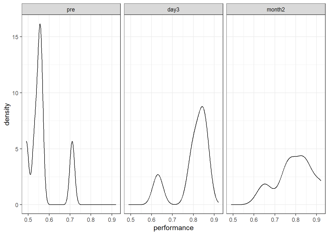
Figure 6.1: Density plots of performance at each time point
The density plots look a little 'lumpy'. Remember that in our sample, there are only six data points per condition, so the plots are unlikely to be representative of the true (population) distribution of scores!
6.4.5 Plot the means
# load the ggpubr package
library(ggpubr)

# use ggline() to plot the means
discriminate_long %>%
  ggline(x = "time" , y = "performance", add = "mean") +
  ylab("Performance") +
  ylim(c(0,1))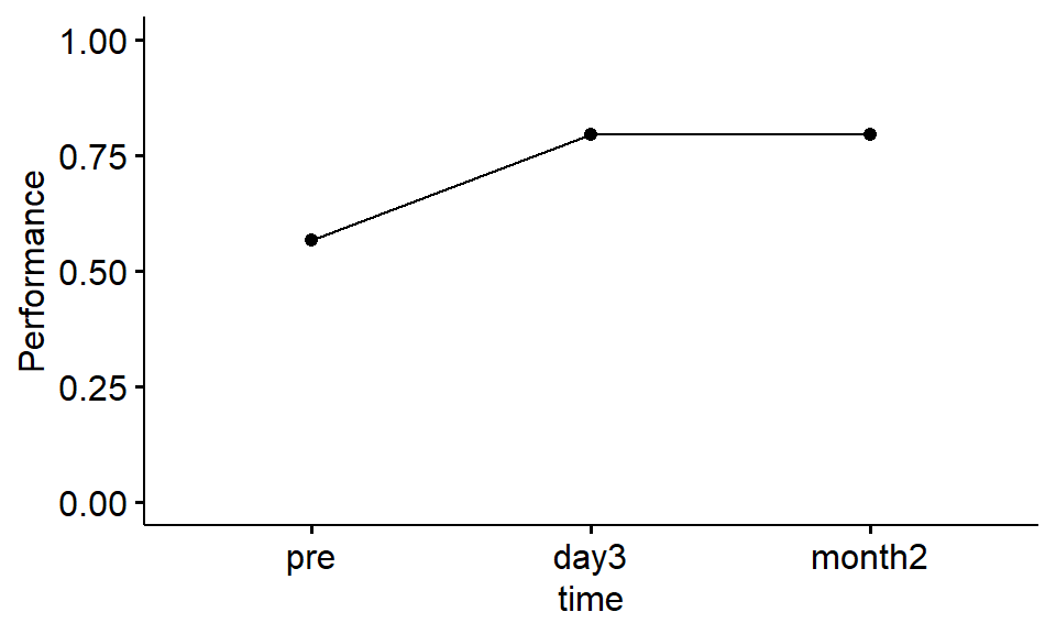
Figure 1.2: Mean proportion correct at each time point
Previously, we used desc_stat = "mean_se" to add errorbars to the plot. Doing so here would add error bars representing the standard error of the mean to each of the points in the plot. These are appropriate for between-subjects designs, but for within-subjects designs, these are not as appropriate. Refer to the Further Knowledge section at the end of the worksheet to see how to add within-subject error bars (and see Morey, 2008, for more detail).
discriminate_long %>%
  ggplot(aes(x = time , y = performance)) +
  stat_summary(fun = mean, geom = "point") +
  stat_summary(aes(group = 1), fun = mean, geom = "line") +
  ylab("Performance") +
  ylim(c(0,1)) +
  theme_classic()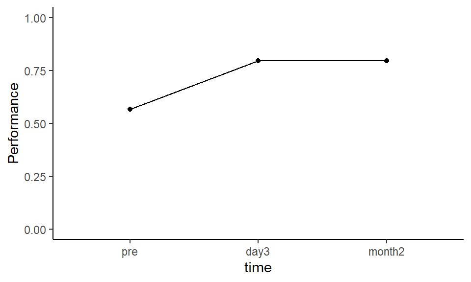
Figure 3.1: Mean proportion correct at each time point
Exercise 6.6 Describe the trend shown in the line plot:
- Between
preandday3, performance appeared to - Between
preandmonth2, performance appeared to - Between
day3andmonth2, performance appeared to
6.4.6 Descriptives: Mean of each condition
Obtain the mean proportion correct at each time point using summarise():
| time | M |
|---|---|
| pre | 0.5666667 |
| day3 | 0.7966667 |
| month2 | 0.7966667 |
6.4.7 Bayes factor
The crucial difference in repeated measures designs compared to between-subjects ones concerns the column labeling the participant, ppt.
pptis entered into the model as another predictor variable, i.e., using...+ ppt.pptis specified as a random factor usingwhichRandom =. This means that the model comprising the other predictors in the model will be evaluated relative to the null model containingpptalone.pptis not individually evaluated.
The Bayes factors can be obtained with anovaBF() but can also be obtained (less conveniently) using lmBF().
Using anovaBF():
# library(BayesFactor)

anovaBF(performance ~ time + ppt, whichRandom = "ppt", data = data.frame(discriminate_long))
## Bayes factor analysis
## --------------
## [1] time + ppt : 327.2033 ±0.5%
##
## Against denominator:
## performance ~ ppt
## ---
## Bayes factor type: BFlinearModel, JZSIn the output, the Bayes factor provided is for the model of performance ~ time + ppt vs. the model of performance ~ ppt. The latter is the null model containing only ppt as a predictor variable. The Bayes factor therefore represents evidence for the (unique) effect of time on performance, over and above a model containing ppt only. This differs to between-subject designs, where the null model (in the denominator) is the intercept-only model (representing the grand mean).
Exercise 6.7 The Bayes factor for the effect of time on performance is
This indicates that (select one):
On the basis of the Bayes factor analysis, does neuro-feedback training affect performance in the language learning task?
It is possible to obtain the same result as anovaBF() using lmBF(). Doing so can help us to understand what anovaBF() is doing. Again, we must tell lmBF() that ppt is a random factor, using whichRandom =.
# Equivalent results with lmBF()

# model with time and ppt only
BF_time_ppt <- lmBF(performance ~ time + ppt, whichRandom = "ppt", data = data.frame(discriminate_long))

# model with ppt only
BF_ppt_only <- lmBF(performance ~ ppt, whichRandom = "ppt", data = data.frame(discriminate_long))

# compare model with vs. without time
BF_time_ppt / BF_ppt_only
## Bayes factor analysis
## --------------
## [1] time + ppt : 331.2465 ±0.57%
##
## Against denominator:
## performance ~ ppt
## ---
## Bayes factor type: BFlinearModel, JZSThis produces a Bayes factor of approximately 330. This is equivalent to the BF obtained with anovaBF(), though note that because of the random data sampling methods used to generate the Bayes factors, the value may differ by a small amount.
6.4.8 Follow-up tests
The Bayes factor obtained with anovaBF() above tells us that there's a difference between the means of the conditions, but not which conditions differ from which.
To determine which conditions differ from which, filter the data for the conditions of interest, then use anovaBF() in exactly the same way as before, but this time with relevant filtered data.
6.4.8.1 Pre vs. day3 conditions
# pre vs. day3
# filter the data for the relevant conditions
pre_v_day3 <- discriminate_long %>% filter(time == "pre" | time == "day3")
#
# compare the means of the conditions, using anovaBF()
anovaBF(performance ~ time + ppt, whichRandom = "ppt", data = data.frame(pre_v_day3))
## Bayes factor analysis
## --------------
## [1] time + ppt : 83.12013 ±3.12%
##
## Against denominator:
## performance ~ ppt
## ---
## Bayes factor type: BFlinearModel, JZS- The Bayes factor for the comparison of mean performance in the
preandday3conditions is . Note. Your BF may differ slightly from the one above due to the random sampling methods anovaBF() uses. - This indicates that there is evidence for between the performance in the
preandday3conditions. - Performance at
day3was than performancepretraining.
6.4.8.2 Pre vs. month2 conditions
# pre vs. month2
# filter the data for these conditions
pre_v_month2 <- discriminate_long %>% filter(time == "pre" | time == "month2")
#
# compare the means of the conditions, using anovaBF()
anovaBF(performance ~ time + ppt, whichRandom = "ppt", data = data.frame(pre_v_month2))
## Bayes factor analysis
## --------------
## [1] time + ppt : 54.19199 ±0.97%
##
## Against denominator:
## performance ~ ppt
## ---
## Bayes factor type: BFlinearModel, JZS- The Bayes factor for the comparison of mean performance in the
preandmonth2conditions is - This indicates that there is evidence for between the mean performance in the
preandmonth2conditions. - Performance at
month2was than performancepretraining.
6.4.8.3 day3 vs. month2 conditions
# day3 vs. month2
# filter the data for these conditions
day3_v_month2 <- discriminate_long %>% filter(time == "day3" | time == "month2")
#
# compare the means of the conditions, using anovaBF()
anovaBF(performance ~ time + ppt, whichRandom = "ppt", data = data.frame(day3_v_month2))
## Bayes factor analysis
## --------------
## [1] time + ppt : 0.4709756 ±1.91%
##
## Against denominator:
## performance ~ ppt
## ---
## Bayes factor type: BFlinearModel, JZS- The Bayes factor for the comparison of mean performance in the
day3andmonth2conditions is - This indicates that there is evidence for between the mean performance in the
day3andmonth2conditions. - Thus, there's no evidence of a difference in performance between the
day3andmonth2conditions.
As before, it's possible to conduct the same comparisons and obtain the same BFs using lmBF():
# pre vs. day3
lmBF(performance ~ time + ppt, whichRandom = "ppt", data = data.frame(pre_v_day3)) /
lmBF(performance ~ ppt, whichRandom = "ppt", data = data.frame(pre_v_day3))

# pre vs. month2
lmBF(performance ~ time + ppt, whichRandom = "ppt", data = data.frame(pre_v_month2)) /
lmBF(performance ~ ppt, whichRandom = "ppt", data = data.frame(pre_v_month2))

# day3 vs. month2
lmBF(performance ~ time + ppt, whichRandom = "ppt", data = data.frame(day3_v_month2)) /
lmBF(performance ~ ppt, whichRandom = "ppt", data = data.frame(day3_v_month2))
## Bayes factor analysis
## --------------
## [1] time + ppt : 80.2486 ±0.63%
##
## Against denominator:
## performance ~ ppt
## ---
## Bayes factor type: BFlinearModel, JZS
##
## Bayes factor analysis
## --------------
## [1] time + ppt : 53.70202 ±0.77%
##
## Against denominator:
## performance ~ ppt
## ---
## Bayes factor type: BFlinearModel, JZS
##
## Bayes factor analysis
## --------------
## [1] time + ppt : 0.4560607 ±1.26%
##
## Against denominator:
## performance ~ ppt
## ---
## Bayes factor type: BFlinearModel, JZS
6.5 Two-way within subjects ANOVA
In a two-way repeated measures or within-subjects ANOVA, there are two categorical independent variables or factors.
When there are multiple factors, the ANOVA is referred to as factorial ANOVA.
For example, if the design has two factors, and each factor has two levels, then we refer to the design as a 2 x 2 factorial design. The first number (2) denotes the number of levels of the first factor. The second number (2) denotes the number of levels of the second factor. If, instead, the second factor had three levels, we'd say we have a 2 x 3 factorial design.
The cells of the design are produced by crossing the levels of one factor with each level of the other factor. If both factors are manipulated within-subjects, then the scores from each cell of the design come from the same group of participants. For example, in a 2 x 2 factorial design, there will be four cells of the design.
6.5.1 Worked Example
Kreysa et al. (2016) analysed RTs to statements made by faces that had different gaze directions - the eyes of the face were either averted to the left, averted to the right, or were looking directly at the participant when the statement was made. RTs were further broken down according to whether the participant had agreed with the statement or not (they responded 'yes' or 'no').
Exercise 6.8 Design check.
What is the first independent variable (or factor) that is mentioned in this design?
How many levels does the first factor have?
What is the second independent variable (or factor) that was mentioned?
How many levels does the second factor have?
What is the dependent variable?
What is the nature of the independent variables?
What type of design is this?
6.5.2 Read in the data
Read in the data from the link below:
https://raw.githubusercontent.com/chrisjberry/Teaching/master/6_gaze_data.csv
gaze <- read_csv('https://raw.githubusercontent.com/chrisjberry/Teaching/master/6_gaze_data.csv')

gaze %>% head()| ppt | gaze_direction | agreement | RT | logRT |
|---|---|---|---|---|
| 1 | averted_left | no | 725.6667 | 6.553344 |
| 1 | averted_left | yes | 787.6667 | 6.615148 |
| 1 | averted_right | no | 621.6667 | 6.389811 |
| 1 | averted_right | yes | 752.6667 | 6.568404 |
| 1 | direct | no | 1001.3333 | 6.829217 |
| 1 | direct | yes | 688.8333 | 6.477116 |
Columns:
ppt: the participant numbergaze_direction: the gaze-direction of the face.agreement: whether the responses made to the statements were 'yes' or 'no'RT: mean response timeslogRT: the log transform of the RT column, i.e.,log(RT)Are the data in long format or wide format?
You can tell this is a repeated measures design and that the data are in long format because a given participant's scores are on multiple rows, and there are multiple scores on the dependent variable (RT) for each participant.
6.5.3 Visualise the data
Reaction time data tend to be positively skewed. As result, Kreysa et al. (2016) analysed the RT data after it had been log transformed.
The log transformed data are in the column logRT.
To see the positive skew, inspect the (untransformed) RTs in RT:
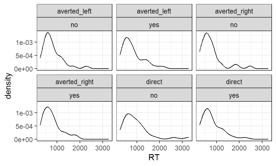
Figure 5.1: Mean RT according to gaze direction and agreement
Now inspect the log transformed RTs in logRT:
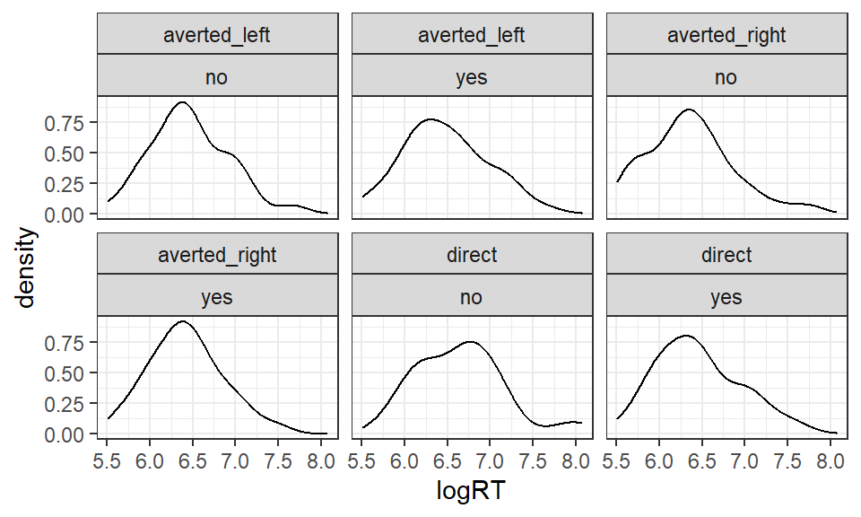
Figure 5.2: Mean logRT according to gaze direction and agreement
- Does the positive skew in the distributions appear to be reduced by the log transformation?
6.5.4 Plot the means
ggline() in the ggpubr package can be used to plot the mean of each condition.
# load the ggpubr package
#library(ggpubr)

# use ggline to plot the means
gaze %>%
  ggline(x = "gaze_direction" , y = "logRT", add = "mean", color= "agreement") +
ylab("Mean log RT") 
Figure 2.3: Mean logRT according to gaze direction and agreement
It appears as if people took longer to respond when the gaze was direct and they said 'no' to the statement that was made.
gaze %>%
  ggplot(aes(x = gaze_direction, y = logRT, color = agreement)) +
  stat_summary(fun = mean, geom = "point") +
  stat_summary(aes(group = agreement), fun = mean, geom = "line") +
  theme_classic()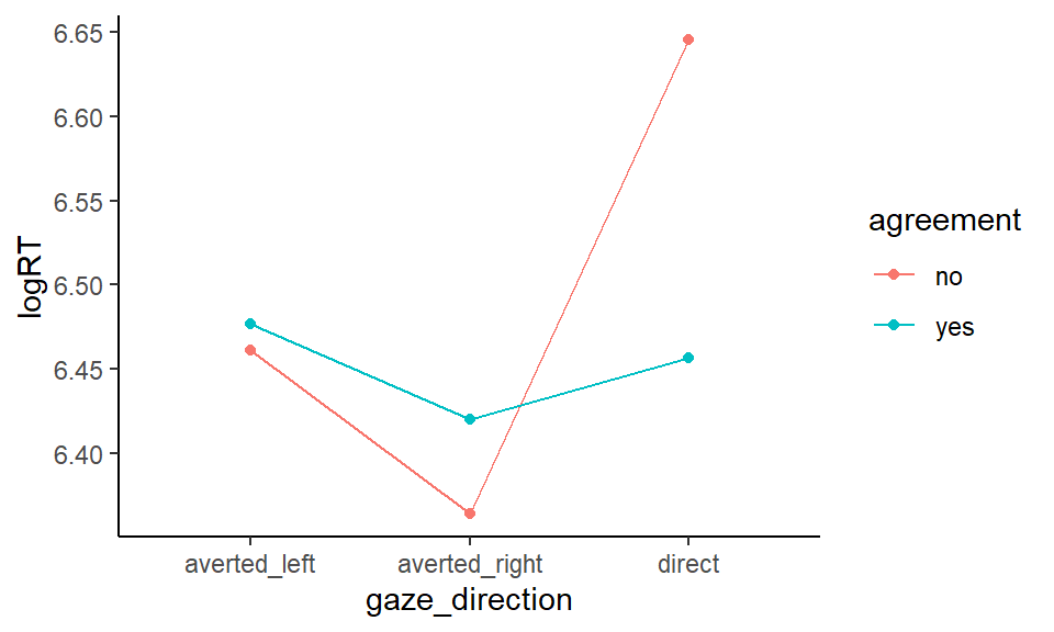
Figure 6.2: Mean logRT according to gaze direction and agreement
6.5.5 Descriptive statistics - mean
To obtain the mean of each condition, use group_by() to group the results of summarise() by the two factors in the design.
Since the log RT values are analysed, we'll obtain the mean of these.
# take the data in gaze
# pipe to group_by()
# group by the gaze_direction and agreement factors
# create a table of the mean of each condition
# and label the column 'M'
gaze %>%
  group_by(gaze_direction, agreement) %>%
summarise(M = mean(logRT))| gaze_direction | agreement | M |
|---|---|---|
| averted_left | no | 6.461225 |
| averted_left | yes | 6.476511 |
| averted_right | no | 6.364156 |
| averted_right | yes | 6.420004 |
| direct | no | 6.645607 |
| direct | yes | 6.456804 |
The mean log RT when participants disagreed with a statement made by a face looking directly at them was (to 2 decimal places) .
6.5.6 Convert participant and categorical variables to factors
Convert the ppt, gaze_direction, and agreement variables to factors so that R will treat them as such in the ANOVA.
# use mutate() to transform
# ppt, gaze_direction and agreement to factors
# and overwrite existing variables
gaze <-
  gaze %>%
  mutate(ppt = factor(ppt),
         gaze_direction = factor(gaze_direction),
         agreement = factor(agreement))

# check changes
gaze %>% head()| ppt | gaze_direction | agreement | RT | logRT |
|---|---|---|---|---|
| 1 | averted_left | no | 725.6667 | 6.553344 |
| 1 | averted_left | yes | 787.6667 | 6.615148 |
| 1 | averted_right | no | 621.6667 | 6.389811 |
| 1 | averted_right | yes | 752.6667 | 6.568404 |
| 1 | direct | no | 1001.3333 | 6.829217 |
| 1 | direct | yes | 688.8333 | 6.477116 |
As before, you could double check that the relevant variable labels in gaze have changed to <fct>.
After using mutate() and factor() above:
In
gaze, what type of variable isppt?In
gaze, what type of variable isgaze_direction?In
gaze, what type of variable isagreement?
6.5.7 Bayes factor
As with between-subjects two-way designs, researchers are typically interested in obtaining three things in a two-way repeated measures ANOVA:
- the main effect of
factor1 - the main effect of
factor2 - the interaction between
factor1andfactor2, i.e., thefactor1*factor2interaction term.
Obtain the Bayes factors for each of the above using anovaBF(). To specify the full model with the interaction, use factor1 * factor2. This will automatically specify a model with the main effects of factor1 and factor2, in addition to the interaction term:
As before, add ppt to the model using ...+ ppt, and tell R it is a random factor using whichRandom = ppt.
# obtain BFs for the anova
BFs_gaze <-
  anovaBF(logRT ~ gaze_direction*agreement + ppt,
          whichRandom = "ppt",
          data = data.frame(gaze) )

# look at BFs
BFs_gaze
## Bayes factor analysis
## --------------
## [1] gaze_direction + ppt : 26.24833 ±0.77%
## [2] agreement + ppt : 0.2682851 ±1.32%
## [3] gaze_direction + agreement + ppt : 7.485079 ±1.89%
## [4] gaze_direction + agreement + gaze_direction:agreement + ppt : 48.65241 ±8.65%
##
## Against denominator:
## logRT ~ ppt
## ---
## Bayes factor type: BFlinearModel, JZSInterpretation of the output is similar as with two-way between-subjects ANOVA (Session 3). Notice, however, that ppt is included in each of models, and the comparison of each model is not against the intercept-only model as it was with between-subjects factorial ANOVA. Because this is a repeated measures design, each model is compared against a null model containing only ppt as a predictor.
6.5.7.1 Main effect of gaze_direction
The main effect of gaze direction:
## Bayes factor analysis
## --------------
## [1] gaze_direction + ppt : 26.24833 ±0.77%
##
## Against denominator:
##   logRT ~ ppt
## ---
## Bayes factor type: BFlinearModel, JZS- RTs tended between
gaze_directionconditions, BF = .
6.5.7.2 The main effect of agreement
## Bayes factor analysis
## --------------
## [1] agreement + ppt : 0.2682851 ±1.32%
##
## Against denominator:
##   logRT ~ ppt
## ---
## Bayes factor type: BFlinearModel, JZS- RTs tended between
agreementconditions, BF = .
6.5.7.3 The gaze_direction x agreement interaction
## Bayes factor analysis
## --------------
## [1] gaze_direction + agreement + gaze_direction:agreement + ppt : 6.499919 ±8.85%
##
## Against denominator:
##   logRT ~ gaze_direction + agreement + ppt
## ---
## Bayes factor type: BFlinearModel, JZS- There an interaction between
gaze_directionandagreement, BF = .
6.5.8 Follow up comparisons
Given the evidence for an interaction, Kreysa et al. (2016) conducted pairwise comparisons to compare "yes" and "no" responses in each gaze direction condition.
This can be achieved by filtering the data for each gaze direction condition, and then using anovaBF() to compare scores in each agreement condition.
If there were no evidence for the interaction, we wouldn't conduct further comparisons.
6.5.8.1 averted_left
# filter data for averted_left condition
averted_left <-
  gaze %>%
  filter(gaze_direction == "averted_left")

# use anovaBF() to compare the agreement conditions
anovaBF(logRT ~ agreement + ppt, whichRandom = "ppt", data = data.frame(averted_left))
## Bayes factor analysis
## --------------
## [1] agreement + ppt : 0.2508754 ±1.13%
##
## Against denominator:
## logRT ~ ppt
## ---
## Bayes factor type: BFlinearModel, JZSThere was substantial evidence for between the mean log RTs made to "yes" and "no" responses in the averted_left condition, BF = .
6.5.8.2 averted_right
# filter data for averted right condition
averted_right <-
  gaze %>%
  filter(gaze_direction == "averted_right")

# use anovaBF() to compare the agreement conditions
anovaBF(logRT ~ agreement + ppt, whichRandom = "ppt", data = data.frame(averted_right))
## Bayes factor analysis
## --------------
## [1] agreement + ppt : 0.5976419 ±41.59%
##
## Against denominator:
## logRT ~ ppt
## ---
## Bayes factor type: BFlinearModel, JZSThe Bayes factor comparing the mean log RTs to "yes" and "no" responses in the averted_right condition was inconclusive, BF = , although there was more evidence for the null hypothesis of there being no difference between conditions.
6.5.8.3 direct
# filter data for direct condition
direct <-
  gaze %>%
  filter(gaze_direction == "direct")

# use anovaBF() to compare the agreement conditions
anovaBF(logRT ~ agreement + ppt, whichRandom = "ppt", data = data.frame(direct))
## Bayes factor analysis
## --------------
## [1] agreement + ppt : 33.9724 ±0.96%
##
## Against denominator:
## logRT ~ ppt
## ---
## Bayes factor type: BFlinearModel, JZS- There was substantial evidence for between the mean log RTs made to "yes" and "no" responses in the
directcondition, BF = . - RTs tended to be longer in the direct condition when participants made a response.
6.6 Exercise: two-way mixed ANOVA
Exercise 6.9 Mixed ANOVA
When one of the factors is manipulated within-subjects and the other is manipulated between-subjects, the design is said to be a mixed design. It is also sometimes called a split-plot design.
Hammel and Chan (2016) looked at the duration (in seconds) that participants were able to balance on a balance-board on three successive occasions (trials). There were three groups of participants: one group (counterfactual) engaged in counterfactual thinking, another group (prefactual) engaged in prefactual thinking, and another group (control) engaged in an unrelated thinking task.
The data (already in long format) are located at the link below:
https://raw.githubusercontent.com/chrisjberry/Teaching/master/6_improve_long.csv
1. Create a line plot of trial vs. duration. Represent each group as a separate line.
- Balance duration seems highest in the group.
- Balance duration seems lowest in the group.
- Balance duration generally appears to across trials.
- convert
pptand the columns labeling the levels of the independent variables to factors. - use
ggline()in theggpubrpackage to create the line plot.
2. Bayes factors
- The main effect of group: BF =
- The main effect of trial: BF =
- The
groupxtrialinteraction:
Note. It may take a short while for anovaBF() to determine the BFs. The processing time increases for more complex designs, especially those with repeated measures.
# convert ppt and independent variables to factors
balance <-
  balance %>%
  mutate(ppt = factor(ppt),
         group = factor(group),
         trial = factor(trial))

# anovaBF
#library(BayesFactor)
bfs <- anovaBF(duration ~ ppt + group + trial, whichRandom = "ppt", data = data.frame(balance))

# main effect of group
bfs[1]

# main effect of trial
bfs[2]

# group*trial interaction
bfs[4] / bfs[3]

# You'll notice there is a large amount of error on the interaction term
# If you have time to wait, then we can recompute the BF with a larger number of iterations,
# which should reduce the error. The BFs come out very similarly, but with smaller error.
# Try this:
# bfs2 <- recompute(bfs, iterations = 100000)
# bfs2[1]
# bfs2[2]
# bfs2[4]/bfs2[3]
4. Follow up comparisons.
Conduct follow-up comparisons to investigate the interaction further. Note, we wouldn't usually do this because there was evidence against there being an interaction between trial and group. In statistical terms, this means that the effect of trial is the same in each group, so there's no need to dig deeper into the data. Instead, the following is a pedagogical exercise only.
Assuming there were an interaction, one approach to investigating it is, for each group, to conduct a one-way ANOVA to determine the effect of trial on duration. This is called a simple effects analysis. This is where we assess the effect of trial at each level of the second factor, in this case group.
Conduct three one-way repeated measures ANOVAs, comparing duration across the three types of trial in each group.
Prefactual group: There's substantial evidence for the effect of
trialonduration, BF = .Counterfactual group: There's substantial evidence for the effect of
trialonduration, BF = .Control group: There's insufficient evidence for the effect of
trialonduration, BF = .
- Use
filter()to subset the data for each group. - Use
anovaBF()to conduct a one-way repeated measures ANOVA for each group.
# filter rows corresponding to prefactual group
prefactual <- balance %>% filter(group == "prefactual")
#
# one-way ANOVA, comparing trial_1, trial_2, trial_3
anovaBF(duration ~ trial + ppt, whichRandom = "ppt", data = data.frame(prefactual))


# filter rows corresponding to counterfactual group
counterfactual <- balance %>% filter(group == "counterfactual")
#
# one-way ANOVA, comparing trial_1, trial_2, trial_3
anovaBF(duration ~ trial + ppt, whichRandom = "ppt", data = data.frame(counterfactual))


# filter rows corresponding to control group
control <- balance %>% filter(group == "control")
#
# one-way ANOVA, comparing trial_1, trial_2, trial_3
anovaBF(duration ~ trial + ppt, whichRandom = "ppt", data = data.frame(control))
6.7 Further knowledge - within-subject errorbars
Here I show you how to plot the means with within-subject error bars (following Morey, 2008) for the first dataset in the worksheet discriminate_long.
I use summarySEwithin() from the Rmisc package for this. The functions from this package have similar names to other tidyverse functions, which can lead to problems/conflicts later. For that reason, I unload Rmisc after using the functions from it, then reload the tidyverse.
# within-subjects error bars

# load Rmisc package for the summarySEwithin() function
library(Rmisc)

# get within-subject intervals
# can also specify between-subjects vars with 'betweenvars = '
intervals_RM <-
  summarySEwithin(discriminate_long,
                  measurevar = "performance",
                  withinvars = "time",
                  idvar = "ppt")

# look at what's produced
# intervals_RM

# select time, performance and se columns
# rename 'performance' to M
intervals_RM <-
  intervals_RM %>%
  select(time, performance, se) %>%
  dplyr::rename(M = performance,
                SE = se)

# compare with between subject intervals (they should be larger)
# summarySE(discriminate_long, measurevar = "performance", groupvars = "time")

# unload the Rmisc package due to conflicts with other packages
detach("package:Rmisc", unload = TRUE)

# now use the M and within-subjects SE to create a plot of means
intervals_RM %>%
  ggplot(aes(x = time, y = M)) +
  geom_point() +
  geom_errorbar(aes(ymin = M - SE, ymax = M + SE), width=.2,
                 position = position_dodge(.9)) +
  theme_classic()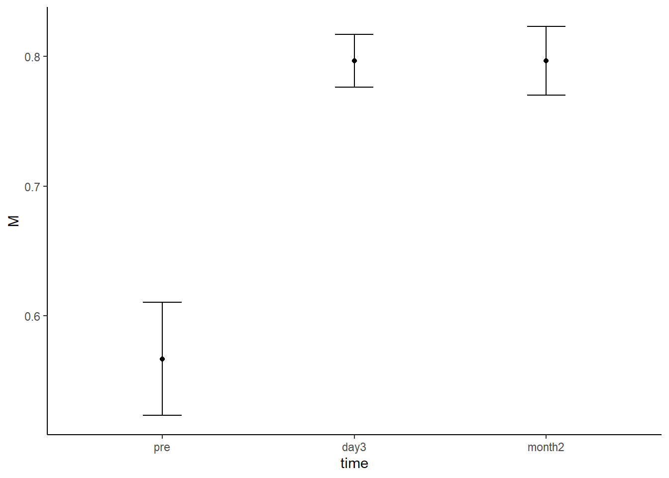
Figure 6.3: Mean proportion correct at each time point. Error bars represent within-subjects standard error of the mean
6.8 Further knowledge - R-squared
It's possible to obtain R2 for the ANOVA model as we have done previously, by specifying the model with lm(), and then using glance():
For the one-way repeated measures ANOVA:
# specify full model with ppt and time using lm()
ppt_and_time <- lm(performance ~ ppt + time, data = discriminate_long)

# look at R-squared
glance(ppt_and_time)- This produces an R2 value, which is relatively high, R2 = (non-corrected, as a proportion, to two decimal places).
This value of R2 is, however, for the full ANOVA model, which includes the random factor ppt too. Given that we are interested in the R2 associated with time only, we need to work out the change in R2 as a result of adding time to the model containing ppt.
To do this, obtain R2 for the model with ppt alone:
# specify model with ppt only using lm()
ppt_alone <- lm(performance ~ ppt, data = discriminate_long)

# make sure the broom package is loaded
#library(broom)

# look at R-squared
glance(ppt_alone)- R2 for the model with
pptalone =
The R2 associated with the time factor can be calculated as the difference in R2 values for the models:
- Thus, R2 for the
timefactor =
The value of R2 that we have calculated for time is the one that we would provide in a journal article, and could be reported as a measure of effect size.
In the literature, this R2 value actually goes by the name generalised eta-squared, and is the recommended measure of effect size for repeated measures designs (see Bakeman, 2005, for more details).
To calculate generalised eta-squared for each factor and the interaction term in a repeated measures ANOVA, each model in the design must be separately specified with lm(). The change in R2 value for each factor and the interaction must then be separately determined, by subtracting the relevant R2 value:
# specify each model in the design
gaze_ppt_only <- lm(logRT ~ ppt, data = gaze)
gaze_ppt_agreement <- lm(logRT ~ ppt + agreement, data = gaze)
gaze_ppt_gaze <- lm(logRT ~ ppt + gaze_direction, data = gaze)
gaze_ppt_agreement_gaze <- lm(logRT ~ ppt + agreement + gaze_direction, data = gaze)
gaze_ppt_agreement_gaze_interaction <- lm(logRT ~ ppt + agreement + gaze_direction + agreement*gaze_direction, data = gaze)

# work out change in R-squared (equivalent to Generalised Eta Squared or ges)
glance(gaze_ppt_agreement)$r.squared - glance(gaze_ppt_only)$r.squared # ges for agreement
glance(gaze_ppt_gaze)$r.squared - glance(gaze_ppt_only)$r.squared # ges for gaze_direction
glance(gaze_ppt_agreement_gaze_interaction)$r.squared - glance(gaze_ppt_agreement_gaze)$r.squared # ges for interaction
This is clearly quite cumbersome, and potentially error prone. For this reason, you may wish to use a package that will determine generalised eta-squared automatically, such as the afex package, which stands for Analysis of Factorial EXperiments. The package performs an ANOVA using frequentist methods, but provides generalised eta squared by default in the output.
library(afex)

# use the afex package to run a 2 x 2 ANOVA
# id is the column of participant identifiers ("ppt")
# dv is the dependent variable ("logRT")
# within specifies the within-subjects factors
anova2way <- afex::aov_ez(id = c("ppt"),
                          dv = c("logRT"),
                          within = c("agreement","gaze_direction"), # two factors
                          data = gaze)
The ges column provides the generalised eta squared values for each effect.
The afex package can also be used to obtain generalised eta squared for one-way between-subjects ANOVA designs.
For the one-way between-subjects ANOVA performed on the affect_data in Session 3:
# Read in the data
affect_data <- read_csv('https://raw.githubusercontent.com/chrisjberry/Teaching/master/3_affect.csv')

# use mutate() to convert the group variable to a factor
# store the changes back in affect_data
# (i.e., overwrite what's already in affect_data)
affect_data <-
  affect_data %>%
  mutate(group = factor(group))

# use the afex package to a one-way ANOVA
# id is the column of participant identifiers ("ppt")
# dv is the dependent variable ("logRT")
# between specifies the between-subjects factor
anova1way <- afex::aov_ez(id = c("ppt"),
                          dv = c("score"),
                          between = c("group"), # one factor
                          data = affect_data)

# look at output
anova1way
The ges column provides the generalised eta squared value for the effect of group on score. The value (0.052) matches the value of R2 we found using lm() and glance(). Generalised eta squared is the same as R2 in this design.
The afex package can also be used to obtain generalised eta squared for two-way between-subjects ANOVA designs.
For the two-way between-subjects ANOVA performed on the resilience_data in Session 3:
# read in the data
resilience_data <- read_csv('https://raw.githubusercontent.com/chrisjberry/Teaching/master/3_resilience_data.csv')

# use mutate() and factor() to convert
# resilience and adversity to factors
# add a ppt column
resilience_data <-
  resilience_data %>%
  mutate(resilience = factor(resilience),
         adversity  = factor(adversity),
         ppt = c(1:n()))

# use the afex package to a two-way ANOVA
# id is the column of participant identifiers ("ppt")
# dv is the dependent variable ("logRT")
# between specifies the between-subjects factor
anova2bet <- afex::aov_ez(id = c("ppt"),
                          dv = c("distress"),
                          between = c("resilience","adversity"), # two factors
                          data = resilience_data)

anova2bet
The generalised eta squared values are in the column ges.
6.9 Summary
- To analyse repeated measures data with ANOVA, the data must be in long format.
- Convert from wide to long format using
pivot_longer(). - Convert the columns containing the participant identifier (e.g.,
ppt) and independent variables to factors usingfactor(). - Add
pptas a predictor inanovaBF(), and specify as a random factor usingwhichRandom = "ppt". - Bayes factors given by
anovaBF()compare each model against a null model withpptonly (as a random factor), rather than the intercept-only model (as was the case in between-subjects designs). - Conduct follow-up tests using
anovaBF()if there's evidence for an interaction.
6.10 References
Bakeman, R. (2005). Recommended effect size statistics for repeated measures designs. Behavior Research Methods, 37(3), 379-384. https://doi.org/10.3758/BF03192707
Chang, M., Ando, H., Maeda, T., Naruse, Y. (2021). Behavioral effect of mismatch negativity neurofeedback on foreign language learning. PLoS ONE, 16(7): e0254771. https://doi.org/10.1371/journal.pone.0254771
Hammell, C., Chan, A.Y.C. (2016). Improving physical task performance with counterfactual and prefactual thinking. PLoS ONE, 11(12): e0168181. doi:10.1371/journal.pone.0168181
Kreysa, H., Kessler, L., Schweinberger, S.R. (2016). Direct Speaker Gaze Promotes Trust in Truth-Ambiguous Statements. PLoS ONE, 11(9): e0162291. doi:10.1371/journal.pone.0162291
Morey, R. D. (2008). Confidence intervals from normalized data: A correction to Cousineau (2005). Reason, 4(2), 61-64.
Rouder, J. N., Morey, R. D., Speckman, P. L., & Province, J. M. (2012). Default Bayes factors for ANOVA designs. Journal of Mathematical Psychology, 56(5), 356-374.