Session 3 ANOVA: between-subjects designs

Chris Berry
2025

3.1 Overview

Slides for the lecture accompanying this worksheet are on the DLE.
R Studio online Access here using University log-in

So far we have used regression where both the outcome and predictor are continuous variables.

When all the predictor variables in a regression are categorical, the analysis is called ANOVA, which stands for Analysis Of VAriance. Here we consider two types of ANOVA for between-subjects designs: one-way ANOVA and two-way ANOVA. We will consider other types in future sessions (e.g., for within-subjects/repeated measures designs).

3.2 One-way between subjects ANOVA

A one-way between subjects ANOVA is used to compare the scores from a dependent variable across different groups of individuals. For example, do mood scores differ between three groups of individuals, where each group undergoes a different type of therapy as treatment?

one-way means that there is one independent variable, for example, type of therapy.
Independent variables are also called factors in ANOVA.
A factor is made up of different levels. Type of therapy could have three levels: CBT (Cognitive Behavioural Therapy), EMDR (Eye Movement Desensitisation and Reprocessing), and Control.
between subjects means that a different group of participants gives us mood scores for each level of the independent variable. For example, if type of therapy is manipulated between-subjects, one group receives CBT, another group receives EMDR, and another group are the control group. Each participant provides exactly one score.

3.2.1 Worked Example

What is the effect of viewing pictures of different aesthetic value on a person's mood? To investigate, Meidenbauer et al. (2020) showed three groups of participants pictures of urban environments that were either very low in aesthetic value (n = 102), low in aesthetic value (n = 100), or high (n = 104). Participants' change in State Trait Anxiety Inventory (STAI: a measure of negative symptoms such as upset, tense, worried) as a result of viewing the pictures was measured.

Exercise 3.1 Design check.

What is the independent variable (or factor) in this design?
How many levels does the factor have?
What is the dependent variable?
What is the nature of the independent variable?
Is the independent variable manipulated within- or between-subjects?

3.2.2 Read in the data

Read in the data at the link below and store in affect_data. Preview the data using head().

https://raw.githubusercontent.com/chrisjberry/Teaching/master/3_affect.csv

(Note. The data in are taken from the Urban condition of Meidenbauer et al. (2020, Experiment 1). The data are publicly available through the links in their article. The variable names have been changed here for clarity.)

# Read in the data
affect_data <- read_csv('https://raw.githubusercontent.com/chrisjberry/Teaching/master/3_affect.csv')

# look at the first 6 rows
affect_data %>% head()

Key variables of interest in affect_data:

group: the aesthetic value group, with levels VeryLow, Low and High
score: the change in STAI score. Higher scores indicate fewer negative symptoms after viewing the images (i.e., improvement in mood).

Notice that the group column is by default read into R as a character variable (that's what the label <chr> means in the output). This is because the levels of group have been recorded in the dataset as words e.g., "VeryLow".

3.2.3 Convert the independent variable to a factor

To enable us to use the group column in an ANOVA, we need to tell R that group is a factor. Use mutate() and factor() to convert group to a factor.

# use mutate() to convert the group variable to a factor
# store the changes back in affect_data 
# (i.e., overwrite what's already in affect_data)

affect_data <-
  affect_data %>% 
  mutate(group = factor(group))

mutate() can be used to change variables or create new ones.

The code mutate(group = factor(group)) means:

group =: create a variable called group. Because group already exists in affect_data it will be overwritten.
factor(group): convert the group variable to a factor.

If we'd have used:

factor(group, levels = c("VeryLow","Low","High"))

instead of

factor(group)

this would mean that the levels of group will additionally be ordered according to the order in levels.

This can be useful when plotting the data.

Check that the variable label for group has now changed from <chr> to <fct> (i.e., a factor) by looking at the dataset again.

affect_data

3.2.4 n of each group

Use group_by() and count() to obtain the number of participants in each group:

# use group_by() to group the output by 'group' column, 
# then obtain number of rows in each group with count()

affect_data %>% 
  group_by(group) %>% 
  count()

How many participants were there in the VeryLow aesthetic value group?
How many participants were there in the Low aesthetic value group?
How many participants were there in the High aesthetic value group?

3.2.5 Visualise the data

The way the data are distributed in each group can be inspected with histograms or density plots:

# Histogram of scores in each group 
# Use facet_wrap(~group) to create a separate
# panel for each group

affect_data %>% 
  ggplot(aes(score)) +
  geom_histogram() + 
  facet_wrap(~group)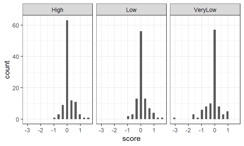

Figure 1.2: Histogram of scores in each aesthetic value group

To produce density plots, swap geom_histogram() with geom_density().

The spread of scores in each group appears relatively similar, suggesting the assumption of homogeneity of variance in ANOVA, may be met. The distributions are reasonably symmetrical, and, aside from the very high number of 0 scores in each group (indicative of zero change in STAI score in a large number of individuals), the data appear approximately normally distributed. In practice, ANOVA is considered reasonably robust against violations of the test's assumptions (see e.g., Glass et al. 1972, Schmider et al., 2010).

3.2.6 Plot the means

Visualise the data further by obtaining a plot of the mean score in each group.

The package ggpubr can produce high quality plots with ease. Using ggerrorplot() in ggpubr:

# load the ggpubr package
library(ggpubr)

# plot the mean of each group 
# specify desc_stat = "mean_se" to 
# add error bars representing the standard error 

affect_data %>% 
  ggerrorplot(x = "group" , y = "score", desc_stat = "mean_se") +
  xlab("Aesthetic value group")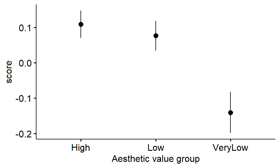

Figure 3.1: Mean change in STAI score across aesthetic value groups (error bars indicate SE)

From inspection of the means:

Which aesthetic value group has the greatest improvement in STAI score?
Which aesthetic value group has the lowest improvement in STAI score?
Did STAI scores appear to worsen (i.e., be below zero) in any group as a result of viewing the images?

As with plots generated in ggplot(), the figure can be enhanced by adding further code, e.g., try adding the line:

+ ylab("Change in STAI (negative symptoms)")

Beneath the surface, ggpubr uses ggplot() to make graphs.

Other types of plot are available in ggpubr, see e.g.:

Errorplots: ?ggerrorplot()
Boxplots: ?ggboxplot()
Violin plots: ?ggviolin()

I encourage you to play around to find clear and effective ways to visualise your data!

To see more types of plot: help(package = ggpubr)

It is of course possible to create the same figure using ggplot:

# pipe data to ggplot
# use stat_summary() to plot the mean
# and again to plot errorbars
affect_data %>% 
  ggplot(aes(x=group,y=score))+
  stat_summary(fun="mean") +
  stat_summary(fun.data = mean_se, geom = "errorbar") +
  theme_classic()

## Warning: Removed 3 rows containing missing values or values outside the scale range
## (`geom_segment()`).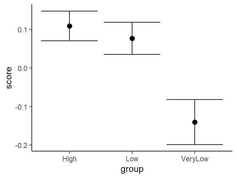

Figure 3.2: Mean change in STAI score across aesthetic value groups (error bars indicate SE)

3.2.7 Descriptives: Mean of each group

Use summarise() and group_by() to obtain the mean (M) in each group:

affect_data %>% 
  group_by(group) %>% 
  summarise(M = mean(score))

The mean score in the High group is (to 2 decimal places)
The mean score in the Low group is (to 2 decimal places)
The mean score in the VeryLow group is (to 2 decimal places)

The formula for the standard error of the mean is \(SD / \sqrt{n}\). We can therefore obtain the standard error of the mean for each group as follows:

affect_data %>% 
  group_by(group) %>% 
  summarise(SE = sd(score) / sqrt( n() ))

To show the mean and SE in the same output:

affect_data %>% 
  group_by(group) %>% 
  summarise( M = mean(score), 
             SE = sd(score) / sqrt( n() ) )

3.2.8 Bayes factor

A Bayes factor can be obtained for the one-way ANOVA model using anovaBF(). The model we specify is of score on the basis of group (i.e., score ~ group). The BF will tell us how much more likely the model (with different three groups) is than an intercept-only model, in which all the scores are treated as coming from one large group. In other words, the BF will tell us whether we have evidence for an effect of aesthetic appeal on the STAI scores or not.

To obtain the BF for the one-way ANOVA model, use anovaBF():

# ensure BayesFactor package is loaded
# library(BayesFactor)

# obtain the BF for the ANOVA model with lmBF()
anovaBF( score ~ group, data = data.frame(affect_data) )

## Bayes factor analysis
## --------------
## [1] group : 66.65842 ±0.04%
## 
## Against denominator:
##   Intercept only 
## ---
## Bayes factor type: BFlinearModel, JZS

The Bayes Factor for the model is equal to BF = . This indicates that the model is over times more likely than an intercept-only model. There is therefore substantial evidence for an effect of the aesthetic value of urban images on changes in STAI scores.

lmBF() in the BayesFactor package can be used in place of lmBF() to produce exactly the same result:

lmBF( score ~ group, data = data.frame(affect_data) )

Remember, this works because ANOVA is a special case of regression.

3.2.9 R²

R² can be reported for ANOVA models as a measure of effect size. As with simple and multiple regression, R² represents the proportion of variance explained by the model, where our model is that the scores come from distinct groups of individuals (three groups in our example) with different means.

To obtain R², first use lm() to specify the model, then use glance() from the broom package:

# specify and store the anova
anova_1 <- lm(score ~ group, data = affect_data)

# make sure broom package is loaded with library(broom), then
# use glance() with anova_1 
glance(anova_1)

r.squared	adj.r.squared	sigma	statistic	p.value	df	logLik	AIC	BIC	deviance	df.residual	nobs
0.0523547	0.0460996	0.4743	8.369943	0.0002896	2	-204.4377	416.8754	431.7697	68.16302	303	306

Adjusted R² (as a percentage, to two decimal places) = %, which represents the percentage of the variance in the change in STAI scores that is explained by the affect value of an image. (Remember, the values of R² given by glance() are proportions, so need to be multiplied by 100 to get the percentage.)

3.2.10 Follow-up tests

The Bayes factor (66.66) tells us that there's evidence that the means of the three groups differ from one another, but not which groups differ from which.

With three groups, there are three possible pairwise comparisons that can be made:

VeryLow vs. Low
VeryLow vs. High
Low vs. High

To compare scores from two groups, we can use filter() to filter the affect_data so that it contains only the two groups we want to compare. Then use anovaBF() again to compare the scores across groups. The BF will tell us how many times more likely it is that there's a difference between means, compared to no difference.

# Compare scores of VeryLow vs. Low groups
#
# Step 1. Filter affect_data for VeryLow and Low groups only
# Store in 'groups_VeryLow_Low'
groups_VeryLow_Low <- 
  affect_data %>% 
  filter(group == "VeryLow" | group == "Low")
#
# Step 2. Obtain BF for VeryLow vs. Low groups
anovaBF(score ~ group, data = data.frame(groups_VeryLow_Low))


# Compare scores of VeryLow vs. High groups
#
# Step 1. Filter affect_data for VeryLow and High groups only
# Store in 'groups_VeryLow_High'
groups_VeryLow_High <- 
  affect_data %>% 
  filter(group == "VeryLow" | group == "High")
#
# Step 2. Obtain BF for VeryLow vs. Low groups
anovaBF(score ~ group, data = data.frame(groups_VeryLow_High))


# Compare scores of Low vs. High groups
#
# Step 1. Filter affect_data to store Low and High groups only
# Store in 'groups_Low_High'
groups_Low_High <- 
  affect_data %>% 
  filter(group == "Low" | group == "High")
#
# Step 2. Obtain BF for VeryLow vs. Low groups
anovaBF(score ~ group, data = data.frame(groups_Low_High))

## Bayes factor analysis
## --------------
## [1] group : 10.25237 ±0%
## 
## Against denominator:
##   Intercept only 
## ---
## Bayes factor type: BFlinearModel, JZS
## 
## Bayes factor analysis
## --------------
## [1] group : 55.43484 ±0%
## 
## Against denominator:
##   Intercept only 
## ---
## Bayes factor type: BFlinearModel, JZS
## 
## Bayes factor analysis
## --------------
## [1] group : 0.1774611 ±0.06%
## 
## Against denominator:
##   Intercept only 
## ---
## Bayes factor type: BFlinearModel, JZS

To two decimal places:

The BF for the comparison of VeryLow vs. Low groups =
The BF for the comparison of VeryLow vs. High groups =
The BF for the comparison of Low vs. High groups =

Interpretation: The one-way between subjects ANOVA indicated that there was evidence for an effect of aesthetic value on change in STAI scores (BF₁₀ = 66.66). The scores in the VeryLow group were lower than those of the Low (BF₁₀ = 10.25) and High groups (BF₁₀ = 55.43), but scores in the Low and High groups did not differ (BF₁₀ = 0.18). This indicates that STAI scores were lower (i.e., there were more negative symptoms) after viewing images that were very low in aesthetic value, compared to images that were low or high in aesthetic value. Viewing pictures that were low or high in aesthetic value resulted in similar changes in STAI scores.

The | symbol means "or".
The == symbol (an equals sign typed twice) means "is equal to"

So filter(group == "VeryLow" | group == "Low") means "filter the rows of affect_data when the labels in group are equal to VeryLow OR the labels in group are equal to Low

anovaBF() was used to conduct follow-up tests. Because each test had two groups, this is equivalent to a Bayesian t-test, and so the exact same BFs could have been obtained using ttestBF():

# Compare scores of VeryLow vs. Low groups
ttestBF( x = affect_data$score[ affect_data$group=="VeryLow" ], 
         y = affect_data$score[ affect_data$group=="Low" ] )

# compare scores of VeryLow vs. High groups
ttestBF( x = affect_data$score[ affect_data$group=="VeryLow" ], 
         y = affect_data$score[ affect_data$group=="High" ] )

# compare scores of Low vs. High groups
ttestBF( x = affect_data$score[ affect_data$group=="Low" ], 
         y = affect_data$score[ affect_data$group=="High" ] )

3.3 Two-way between-subjects ANOVA

In a two-way ANOVA, there are two categorical independent variables or factors.

When there are multiple factors, the ANOVA is referred to as factorial ANOVA.

For example, if the design has two factors, and each factor has two levels, then we refer to the design as a 2 x 2 factorial design. The first number (2) denotes the number of levels of the first factor. The second number (2) denotes the number of levels of the second factor. If, instead, the second factor had three levels, we'd say we have a 2 x 3 factorial design.

3.3.1 Worked example

What is the role of resilience in the distress experienced from childhood adversities? Beutel et al. (2017) analysed the distress scores from 2,437 individuals who were either low or high in trait resilience and had experienced either low or high levels of childhood adversity.

Exercise 3.2 Design check.

What is the first independent variable (or factor) that is mentioned in this design?
How many levels does the first factor have?
What is the second independent variable (or factor)?
How many levels does the second factor have?
What is the dependent variable?
What is the nature of the independent variables?
What type of design is this?

3.3.2 Read in the data

Read in the data at the link below and store in resilience_data:

https://raw.githubusercontent.com/chrisjberry/Teaching/master/3_resilience_data.csv

# read in the data
resilience_data <- read_csv('https://raw.githubusercontent.com/chrisjberry/Teaching/master/3_resilience_data.csv')

# preview
head(resilience_data)

distress	resilience	adversity	sex	partnership	education	income
0	high	low	1	1	2	2
1	low	low	1	1	1	2
0	high	low	1	2	1	1
0	high	low	1	1	1	2
1	low	low	1	2	2	2
1	high	low	1	1	1	2

distress contains the distress scores. Higher scores indicate greater levels of distress.
resilience labels the levels of childhood adversity ( low or high)
adversity labels the levels of trait resilience ( low or high)

(Note. The data are publicly available, but I have changed some of the variable names for clarity.)

3.3.3 Convert the independent variables to factors

To enable the factors to be used as such in ANOVA, we need to convert them to factors using factor():

# use mutate() and factor() to convert 
# resilience and adversity to factors

resilience_data <- 
  resilience_data %>% 
  mutate(resilience = factor(resilience),
         adversity  = factor(adversity))

3.3.4 n in each group

Obtain the number of participants in each group:

# use count() to obtain the number of rows in the dataset, 
# group_by() both resilience AND adversity
resilience_data %>% 
  group_by(resilience, adversity) %>% 
  count()

resilience	adversity	n
high	high	106
high	low	997
low	high	284
low	low	1050

In a between-subjects factorial design, participants are assigned to groups by crossing the levels of one variable with those of the second variable. Thus, each row labels the level of resilience and level of adversity for that group.

The number of participants in the high resilience, high adversity group is
The number of participants in the high resilience, low adversity group is
The number of participants in the low resilience, high adversity group is
The number of participants in the low resilience, low adversity group is

3.3.5 Visualise the data

The way the data are distributed in each group can be inspected with histograms or density plots.

# Use `facet_wrap(~ resilience * adversity)`
# to plot scores for all combinations of 
# resilience x adversity levels
# use 'labeller = label_both' to label levels by factor name

resilience_data %>% 
  ggplot(aes(distress)) + 
  geom_density() +
  facet_wrap(~ resilience * adversity, labeller = label_both)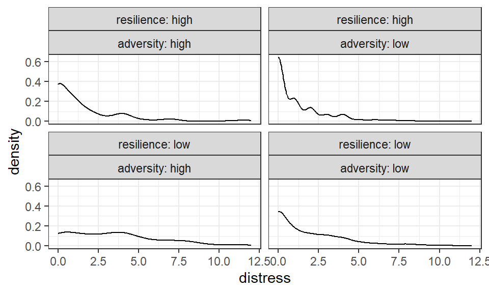

Figure 3.3: Density plots showing distress scores in each group)

Interpretation: The data in each group appear positively skewed - the tail of the distribution goes towards the right (i.e., towards more positive values of distress). Beutel et al. (2017) took no further action and analysed the scores as they were.

3.3.6 Plot the means

Use ggbarplot() in the ggpubr package:

library(ggpubr)

# plot the mean of each group
# use 'desc_stat = "mean_se" to add SE error bars
# use 'position = position_dodge(0.3)' so that points are spaced
resilience_data %>% 
  ggerrorplot(x = "resilience", y = "distress",  color = "adversity",
              desc_stat = "mean_se", 
              position = position_dodge(0.3)) +
  xlab("Resilience") +
  ylab("Distress")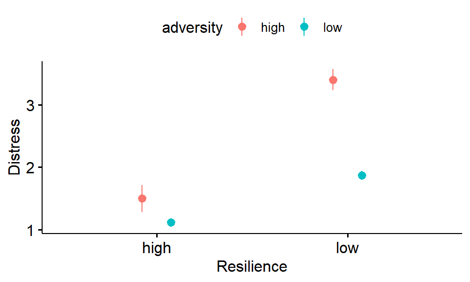

Figure 3.4: Distress as a function of adversity and resilience (error bars indicate SE of the mean)

resilience_data %>% 
  ggplot(aes(x=resilience,y=distress,color=adversity))+
  stat_summary(fun.data = mean_se,geom = "errorbar", position = position_dodge(width=0.5))+
  stat_summary(fun="mean",  position = position_dodge(width=0.5)) +
  theme_classic()

## Warning: Removed 4 rows containing missing values or values outside the scale range
## (`geom_segment()`).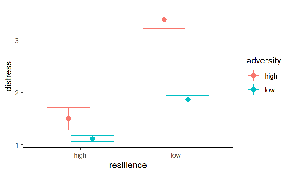

Figure 3.5: Distress as a function of adversity and resilience (error bars indicate SE of the mean)

In a two-way design, researchers look at three things:

The main effect of factor 1: Overall, do scores differ according to the levels of factor 1?
The main effect of factor 2: Overall, do scores differ according to the levels of factor 2?
The interaction between the factors: Is the effect of one factor different at each level of the other factor?

We can get some idea of the main effects and interaction by inspecting the plot of the means:

The main effect of resilience: Overall, distress scores in the high resilience groups appear to be those in the low resilience groups.
The main effect of adversity: Overall, distress scores in the low adversity groups appear to be those in the high adversity groups.
The interaction between resilience and distress: When trait resilience is low rather than high, the effect of adversity on distress appears to be . (Hint: the effect of adversity is indicated by the difference between the red and blue points.)

3.3.7 Bayes factors

Use anovaBF() in the BayesFactor package to obtain Bayes factors corresponding to the main effect of factor 1, the main effect of factor 2, and the interaction between factor 1 and factor 2.

To specify the two-way ANOVA in anovaBF(), use dependent_variable ~ factor1 * factor2.

For the resilience data:

# Obtain the Bayes Factors for the ANOVA model
anova2x2_BF <- anovaBF( distress ~ resilience * adversity, data = data.frame(resilience_data) )

# look at the output
anova2x2_BF

## Bayes factor analysis
## --------------
## [1] resilience                                    : 1.822053e+27 ±0%
## [2] adversity                                     : 7.870878e+25 ±0%
## [3] resilience + adversity                        : 3.454093e+46 ±0.76%
## [4] resilience + adversity + resilience:adversity : 3.317444e+49 ±1.01%
## 
## Against denominator:
##   Intercept only 
## ---
## Bayes factor type: BFlinearModel, JZS

It means 1.82 x 10²⁷. Or 1820000000000000000000000000. A very large number! For more information see: FAQ (Opens a new tab.)

Please take care to notice "e+" or "e-" in the output for your Bayes factors. As you can see, BF₁₀ = 1.82 means something drastically different to BF₁₀ = 1.82 x 10²⁷, and you wouldn't want to make this kind of mistake when drawing statistical inferences!

Each BF in the output compares how likely the model is, compared to an intercept only model:

[1] resilience is the BF for the main effect of resilience. It's how much more likely a model with resilience alone is than an intercept-only model.
[2] adversity is the BF for the main effect of adversity. It's how much more likely a model with adversity alone is than an intercept-only model.
[3] resilience + adversity is the BF for the main effects of resilience and adversity. It's how much more likely a model with main effects of resilience and adversity is than an intercept-only model.
[4] resilience + adversity + resilience:adversity is the BF for the main effects of resilience and adversity and also the interaction between them (resilience:adversity). It's how much more likely a model with main effects of resilience and adversity and also the interaction (resilience:adversity) is than an intercept-only model.

[1] and [2] correspond to the main effects of resilience and adversity, respectively.

To obtain the BF for the interaction, we need to divide [4] by [3]:

# BF for the interaction
anova2x2_BF[4] / anova2x2_BF[3]

## Bayes factor analysis
## --------------
## [1] resilience + adversity + resilience:adversity : 960.4383 ±1.27%
## 
## Against denominator:
##   distress ~ resilience + adversity 
## ---
## Bayes factor type: BFlinearModel, JZS

This BF then tells us whether there's evidence for the addition of an interaction term to a model containing the main effects of each factor. This is the BF for the interaction.

Record the Bayes factors below:

The BF for the main effect of resilience is BF₁₀ = x 10²⁷.
The BF for the main effect of adversity is BF₁₀ = x 10²⁵.
The BF for the resilience and adversity interaction is approximately (to the nearest whole number). Remember, this is the BF you calculated by dividing [4] by [3]. BF₁₀ = .

You'll notice that some of the BFs had ±1.03% or similar next to them in the output. This is the error associated with the BF. It's like saying my height is 185 cm, plus or minus a cm or so. It can be non-zero because generation of the BFs involves random sampling processes. Larger error values mean that the exact same value of the BF won't necessarily be output each time the line of code containing anovaBF() is run, so there's a chance that the BFs in your output differ slightly from those above (particularly for the interaction). This is why I asked you to give your answer to the nearest whole number.

3.3.8 R²

Once again, glance() can be used to obtain R² for the ANOVA model. The model first needs to be specified with lm(). Using factor1 * factor2 when specifying the model is a shortcut, which will automatically specify the full model containing the interaction. Thus, we can use lm(distress ~ resilience * adversity), which is equivalent to lm(distress ~ resilience + adversity + resilience*adversity).

# specify the ANOVA model using lm()
anova2x2 <- lm(distress ~ resilience * adversity, data = resilience_data)

# R^2^
glance(anova2x2)

r.squared	adj.r.squared	sigma	statistic	p.value	df	logLik	AIC	BIC	deviance	df.residual	nobs
0.0963021	0.0951878	2.142569	86.42379	0	3	-5312.959	10635.92	10664.91	11168.93	2433	2437

The adjusted R² of the ANOVA model (to two decimal places, as a percentage) is %, which is the percentage of variance in distress explained by the model.

Rather than report the R² for the overall model in an article, we often would rather report the R² value associated with each of the main effects and interaction.

It is easiest to obtain this by running the ANOVA using the afex package. We'll do this in more detail in Session 6.

# load afex
library(afex)

# add a column to code the ppt in the dataset
resilience_data <- 
  resilience_data %>% 
  mutate(ppt = c(1:n()))

# use the afex package to run a two-way ANOVA
# id is the column of participant identifiers ("ppt")
# dv is the dependent variable ("distress")
# between specifies the between-subjects factor
anova2bet <- afex::aov_ez(id = c("ppt"),
                          dv = c("distress"),
                          between = c("resilience","adversity"), # two factors
                          data = resilience_data)

anova2bet

The R² values are referred to as generalised eta squared. The values for each main effect and the interaction term are in the column ges.

3.3.9 Follow-up comparisons

Given that we have evidence for an interaction, anovaBF() can be used to conduct follow-up comparisons to explore the nature of the interaction. (Note, we would not do this if the BF did not show evidence for the interaction, i.e., if the BF was less than 3.)

The interaction implies the effect of adversity is different in individuals with high resilience, and those with low resilience.

To determine the evidence for the effect of adversity in individuals with high resilience:

# 1. The effect of adversity in individuals with high resilience

# First use filter() to store only 
# the data from the 'high' resilience groups
resilience_high <- 
  resilience_data %>% 
  filter(resilience == "high")

# Then use `anovaBF()` to look at effect of adversity in resilience_high
anovaBF( distress ~ adversity, data = data.frame(resilience_high) )

## Bayes factor analysis
## --------------
## [1] adversity : 1.026598 ±0.02%
## 
## Against denominator:
##   Intercept only 
## ---
## Bayes factor type: BFlinearModel, JZS

To determine the evidence for the effect of adversity in individuals with low resilience:

# 2. The effect of adversity in individuals with low resilience

# First use filter() to store only 
# the data from the 'low' resilience groups
resilience_low <- 
  resilience_data %>% 
  filter(resilience == "low")

# Then use `anovaBF()` to look at effect of adversity in resilience_low
anovaBF( distress ~ adversity, data = data.frame(resilience_low) )

## Bayes factor analysis
## --------------
## [1] adversity : 2.389569e+17 ±0%
## 
## Against denominator:
##   Intercept only 
## ---
## Bayes factor type: BFlinearModel, JZS

This confirms the interaction that is apparent in the plot: There's no evidence for an effect of adversity within high resilience individuals (BF₁₀ = ), but there's substantial evidence for an effect of adversity within low resilience individuals (BF₁₀ = x 10¹⁷), such that levels of distress are greatest when the level of adversity is highest.

Interestingly, this suggests that resilience may have a buffering effect on the distress experienced as a result of childhood adversity (see Beutel et al., 2017, for further discussion).

3.4 Exercise: one-way

Exercise 3.3 One-way ANOVA

The data at the link below are from a study by Bobak et al. (2016). They looked at the face matching performance of individuals with superior face recognition abilities, so called "super recognisers". Their performance was compared to two control groups. In one control group, payment was linked to performance (labelled "motivated_control"). The individuals in the other control group were not paid (labelled "control"). The column face_group contains the labels for each group.

https://raw.githubusercontent.com/chrisjberry/Teaching/master/3_super_data.csv

Conduct a one-way ANOVA to compare the performance across the three groups.

Adapt the code in this worksheet to do the following: Try not to look at the solutions before you've attempted them

1. Read in the data and store in super_data

Ensure the tidyverse package is loaded. See ?read_csv()

super_data <- read_csv('https://raw.githubusercontent.com/chrisjberry/Teaching/master/3_super_data.csv')

# look at the raw data
super_data

2. Convert the independent variable to a factor

See ?mutate() and ?factor()

super_data <- 
  super_data %>% 
  mutate( face_group = factor(face_group) )

3. Obtain n in each group

Pipe the data to group_by() and count()

super_data %>% 
  group_by(face_group) %>% 
  count()

n super recognisers =
n motivated_control =
n control =

4. Produce a histogram of scores in each group

Pipe the data to ggplot() and geom_histogram() and facet_wrap()

super_data %>% 
  ggplot(aes(performance)) +
  geom_histogram() +
  facet_wrap(~face_group)

5. Produce a plot of the means (with SEs) in each group

?ggerrorplot() in the ggpubr package

 # produce means plot

super_data %>% 
  ggerrorplot(x = "face_group", y ="performance", desc_stat = "mean_se") +
  xlab("Group") +
  ylab("Face matching performance")

Face matching performance appears to be highest in the , followed by the , followed lastly by the .

6. Obtain the mean and SE of each group

Use group_by() and summarise()

super_data %>% 
  group_by(face_group) %>% 
  summarise( M  = mean(performance), 
             SE = sd(performance) / sqrt( n() ) )

The mean score of the super_recogniser group is , SE =
The mean score of the motivated_control group is , SE =
The mean score of the control group is , SE =

7. Obtain the Bayes factor for the ANOVA model

The Bayes factor for the model is equal to (to two decimal places) .
This indicates that there is for an effect of the face group on matching performance.

?anovaBF()

anovaBF(performance ~ face_group, data = data.frame(super_data))

8. What is R² for the model?

The adjusted R² for the effect of face group on matching performance is (as a percentage, to two decimal places) %.

obtain the model with lm(), then use glance()

super_anova <- lm(performance ~ face_group, data = super_data)
glance(super_anova)

# multiply the adj.r.squared value by 100 to obtain the percentage
0.301*100

9. Conduct follow-up tests to compare the mean score of each group

Use filter() to create new variables containing the scores of two groups at a time
Then use anovaBF() to compare the scores of each group.

# super_recognisers vs. motivated_control
super_vs_motivated_controls <- 
  super_data %>%
  filter(face_group == "super_recogniser" | face_group == "motivated_control")

anovaBF(performance ~ face_group, data = data.frame(super_vs_motivated_controls))


# super_recognisers vs. control
super_vs_controls <- 
  super_data %>%
  filter(face_group == "super_recogniser" | face_group == "control")

anovaBF(performance ~ face_group, data = data.frame(super_vs_controls))


# motivated_control vs. control
motivated_control_vs_control <- 
  super_data %>%
  filter(face_group == "motivated_control" | face_group == "control")

anovaBF(performance ~ face_group, data = data.frame(motivated_control_vs_control))

# super_recognisers vs. motivated_control
ttestBF(x = super_data$performance[super_data$face_group == "super_recogniser"],
        y = super_data$performance[super_data$face_group == "motivated_control"])

# super_recognisers vs. control
ttestBF(x = super_data$performance[super_data$face_group == "super_recogniser"],
        y = super_data$performance[super_data$face_group == "control"])

# motivated_control vs. control
ttestBF(x = super_data$performance[super_data$face_group == "motivated_control"],
        y = super_data$performance[super_data$face_group == "control"])

The Bayes factor comparing the super_recogniser and motivated_control groups is , indicating a difference between groups.
Face matching performance in the super_recogniser group was than that of the motivated_control group.
The Bayes factor comparing the super_recogniser and control groups is , indicating a difference between groups.
Face matching performance in the super_recogniser group was than that of the control group.
The Bayes factor comparing the motivated_control and control groups is , indicating that there was difference between the scores of each group.

3.5 Exercise: two-way

Exercise 3.4 Two-way ANOVA

Horstmann et al. (2018) looked at whether the type of exchange that people had with a robot would affect how long it would then take for them to switch it off. The type of exchange was either 'functional' or 'social'. Additionally, the researchers looked at the effect of the type of objection that the robot made during the conversation. The robot either voiced an 'objection' to being switched off, or voiced 'no objection'.

Design check.

What is the first independent variable (or factor) that is mentioned in this design?
How many levels does the first factor have?
What is the second independent variable (or factor)?
How many levels does the second factor have?
What is the dependent variable?
What is the nature of the independent variables?
What is the nature of the dependent variable?
What type of design is this?

The robot_data are located at the link below:

https://raw.githubusercontent.com/chrisjberry/Teaching/master/3_robot_data.csv

Adapt the code in this worksheet to do the following:

Conduct a two-way ANOVA to compare the effects of exchange and objection on time. Determine whether there's sufficient evidence for the following:

The main effect of objection: BF₁₀ (to two decimal places) =
The main effect of exchange: BF₁₀ (to two decimal places) =
The interaction between exchange and objection: BF₁₀ (nearest whole number) =

Conduct any follow-up tests concerning the interaction (if necessary).

The effect of exchange when the robot objected: BF₁₀ (to two decimal places) =
The effect of exchange when the robot did not object: BF₁₀ (to two decimal places) =

Interpret the main effects and interaction. What do they mean?

Read in the data to a variable called robot_data
Convert the independent variables to factors using factor()
Examine the distribution of time in each group using geom_histogram() or geom_density() in ggplot()
Obtain summary statistics using group_by(), count() and summarise(mean())
Use a plot from the ggpubr package to create a plot of the means (e.g., ggerrorplot())
Use anovaBF() to obtain the Bayes factors to allow you to assess evidence for the main effects and interaction.
If there's evidence for an interaction, then conduct follow-up tests using anovaBF() or ttestBF()

# ensure following packages have been loaded
# library(tidyverse)
# library(BayesFactor)
# library(ggpubr)

# read the data
robot_data <- read_csv('https://raw.githubusercontent.com/chrisjberry/Teaching/master/3_robot_data.csv')

# convert IVs to factors
robot_data <-
  robot_data %>% 
  mutate(exchange  = factor(exchange),
         objection = factor(objection)) 

# inspect distributions
robot_data %>% 
  ggplot( aes(time) ) + 
  geom_histogram() +
  facet_wrap(~ exchange*objection)

# obtain M and SE each group
robot_data %>% 
  group_by(exchange, objection) %>% 
  summarise( M = mean(time), SE = sd(time)/sqrt(n()) )

# plot of means
robot_data %>% 
  ggerrorplot(x = "objection", y = "time", color = "exchange",
              desc_stat = "mean_se", 
              position = position_dodge(0.3)) +
  xlab("Type of objection") +
  ylab("Switch off time (seconds)") 

# 2x2 ANOVA
BF_robot <- anovaBF( time ~ exchange*objection, data = data.frame(robot_data) )

# look at BFs
BF_robot

# main effect objection
BF_robot[1]

# main effect exchange
BF_robot[2]

# interaction
BF_robot[4] / BF_robot[3]


# Given the evidence for an interaction, conduct further comparisons

# 1. The effect of exchange when the robot objected (i.e., `objection`)

# use filter() to store only 
# the data from the 'objection' groups
robot_objection <- 
  robot_data %>% 
  filter(objection == "objection")

# use `anovaBF()` to look at effect of exchange in the objection groups
anovaBF( time ~ exchange, data = data.frame(robot_objection) )


# 2. The effect of exchange when the robot did not object

# use filter() to store only 
# the data from the 'no_objection' groups
robot_no_objection <- 
  robot_data %>% 
  filter(objection == "no_objection")

# use `anovaBF()` to look at effect of exchange in the no objection groups
anovaBF( time ~ exchange, data = data.frame(robot_no_objection) )


# For the interpretation of main effects:
#
# Obtain M and SE for the main effect of objection
robot_data %>% 
  group_by(objection) %>% 
  summarise( M = mean(time), 
             SE = sd(time)/sqrt(n()) )

# Obtain M and SE for the main effect of exchange
robot_data %>% 
  group_by(exchange) %>% 
  summarise( M = mean(time), 
             SE = sd(time)/sqrt(n()) )

To aid your interpretation of the main effects and interaction, look at the mean of the scores in each group. In which groups is the time taken to switch off the robot longer than others? How does time differ according to type of exchange? How does time differ according to type of objection? Does the effect of exchange seem to be the same at each level of objection?

There was substantial evidence for a main effect of the type of objection on the time it took for a participant to switch off a robot (BF₁₀ = 6.29). Participants took longer when the robot had previously mentioned that it objected to being switched off (M = 10.00 seconds, SE = 2.21), compared to when no objection was mentioned (M = 4.69, SE = 0.37).

There was insufficient evidence for a main effect of the type of exchange, given that the Bayes factor was inconclusive (BF₁₀ = 0.74). Thus, there was no evidence to suggest that the time to switch off a robot differed according to whether the type of exchange was functional (M = 8.69, SE = 2.00) or social (M = 5.54, SE = 0.57).

The main effects should be viewed in light of the substantial evidence for an interaction between exchange and objection (BF₁₀ = 3.28). This indicated that it took people longer to switch the robot off when the exchange had been functional, rather than social, but only if the robot had objected to being switched off (M functional = 14.40, SE = 4.11 vs. M social = 6.19, SE = 1.15). When the robot had not previously objected to being switched off, the times were similar following functional and social exchanges (M functional = 4.28, SE = 0.59, vs. M social = 5.05, SE = 0.48).

Follow-up tests indicated insufficient evidence for the effect of exchange at each level of objection (i.e., BF₁₀s were between 0.33 and 3): The Bayes factor for the effect of exchange when the robot objected was 1.55, and the Bayes factor for the effect of exchange when the robot did not object was 0.47. Thus, although there was evidence for an interaction, the pattern of differences within objection conditions was not confirmed by the follow-up tests.

3.6 Summary

ANOVA is a special case of regression when the predictor variables are entirely categorical.
A one-way between-subjects ANOVA has one independent variable, and separate groups of participants for each level of the independent variable. The test looks at whether the mean scores differ between groups.
A two-way between-subjects ANOVA has two independent variables (factors). Each factor has levels. Researchers examine evidence for the main effect of each factor and their interaction.
The interaction examines the effect of one factor at each level of the other factor.
If there's evidence for an interaction, follow-up comparisons can be performed.
Use anovaBF() to obtain Bayes factors for the main effects and interaction.

3.7 References

Beutel M.E., Tibubos A.N., Klein E.M., Schmutzer G., Reiner I., Kocalevent R-D., et al. (2017) Childhood adversities and distress - The role of resilience in a representative sample. PLoS ONE, 12(3): e0173826. https://doi.org/10.1371/journal.pone.0173826

Glass G.V., Peckham P.D., Sanders J.R. (1972). Consequences of failure to meet assumptions underlying the fixed effects analyses of variance and covariance. Review of Educational Research. 42, 237–288. https://doi.org/10.3102%2F00346543042003237

Horstmann A.C., Bock N., Linhuber E., Szczuka J.M., Straßmann C., Kramer N.C. (2018) Do a robot’s social skills and its objection discourage interactants from switching the robot off? PLoS ONE, 13(7): e0201581. https://doi.org/10.1371/journal.pone.0201581

Meidenbauer, K. L., Stenfors, C. U., Bratman, G. N., Gross, J. J., Schertz, K. E., Choe, K. W., & Berman, M. G. (2020). The affective benefits of nature exposure: What's nature got to do with it?. Journal of Environmental Psychology, 72, 101498. https://doi.org/10.1016/j.jenvp.2020.101498

Schmider E., Ziegler M., Danay E., Beyer L., Bühner M. (2010). Is it really robust? Methodology. 6, 147–151. https://doi.org/10.1027/1614-2241/a000016

Session 3 ANOVA: between-subjects designs

3.1 Overview

3.2 One-way between subjects ANOVA

3.2.1 Worked Example

3.2.2 Read in the data

3.2.3 Convert the independent variable to a factor

3.2.4 n of each group

3.2.5 Visualise the data

3.2.6 Plot the means

3.2.7 Descriptives: Mean of each group

3.2.8 Bayes factor

3.2.9 R2

3.2.10 Follow-up tests

3.3 Two-way between-subjects ANOVA

3.3.1 Worked example

3.3.2 Read in the data

3.3.3 Convert the independent variables to factors

3.3.4 n in each group

3.3.5 Visualise the data

3.3.6 Plot the means

3.3.7 Bayes factors

3.3.8 R2

3.3.9 Follow-up comparisons

3.4 Exercise: one-way

3.5 Exercise: two-way

3.6 Summary

3.7 References

3.2.9 R²

3.3.8 R²