Session 4 Multiple regression: one continuous, one categorical

Chris Berry
2025

4.1 Overview

Slides for the lecture accompanying this worksheet are on the DLE.
R Studio online Access here using University log-in

So far we have looked at simple and multiple regression with continuous variables. (And in the last session, we saw that between-subjects ANOVA was equivalent to a multiple regression in which all the predictors are categorical.)

Here, we look at multiple regression with a mixture of continuous and categorical predictors. Specifically, one predictor is continuous, and the other is a dichotomous categorical variable (i.e., made up of two levels or groups).

This type of analysis can be used to see whether the relationship between two variables is the same or different across groups of individuals. For example, adherence to a particular treatment (e.g., CBT) may be associated with attitudes towards the efficacy of the treatment, but the nature of the association may differ according to the type of psychological disorder a person has (e.g., depressed vs. not depressed).

Thus, in this type of analysis, in addition to looking at the ability of individual predictors to explain an outcome variable, we're able to look at their combined effect in explaining the outcome. This is referred to as an interaction effect. The interaction can tell us whether the relationship between one of the predictors and the outcome differs as a function of the levels of the other predictor variable.

4.2 Worked example

Scientists often research things that are of personal interest to themselves. Do we trust the researcher more when they have some personal investment in what they are researching? Altenmuller et al. (2021) looked at whether participants' trust in the researcher is related to 1) whether they are told that the researcher is personally affected by the research or not affected by their research, and 2) the participant's attitude towards the research topic.

The data from Altenmuller et al.'s (2021) study (Experiment 2) are stored at the link below.

https://raw.githubusercontent.com/chrisjberry/Teaching/master/4_trust_data.csv

The key variables:

trustworthiness: how trustworthy the participant finds the researcher. Higher scores indicate higher levels of trustworthiness.
attitude: the participant's attitude towards the research topic. Higher scores indicate a more positive attitude.
group: whether participants were told that the researcher is personally affected or not_affected by their own research.

The data were made publicly available by the researchers and have been pre-processed (using the researcher's open R code). Only a subset of the data is used here for teaching purposes; variable names have been changed for clarity.

Exercise 4.1 Design check.

What is the outcome variable in this design?
What is the nature of the outcome variable?
What is the name of the continuous predictor variable?
What is the name of the categorical predictor variable?
How many levels of group are there?
When a variable has two levels it is called a variable.

4.3 Read in the data

Read in the data to trust_data

# ensure tidyverse is loaded
# library(tidyverse)

# read in the data
trust_data <- read_csv('https://raw.githubusercontent.com/chrisjberry/Teaching/master/4_trust_data.csv')

# look at the data
trust_data %>% head()

ppt	group	attitude	trustworthiness	credibility	evaluation
1	not_affected	5.714286	4.428571	4.428571	2.583333
2	affected	3.142857	4.285714	4.428571	3.250000
3	not_affected	5.285714	4.428571	4.428571	2.750000
4	not_affected	4.428571	4.642857	3.857143	2.416667
5	affected	6.000000	6.000000	5.285714	2.333333
6	not_affected	3.642857	5.500000	4.571429	2.500000

4.4 Visualise the data

Use a scatterplot to look at the relationship between trustworthiness, attitude and group. Use different colours for each group by specifying colour = group in aes():

trust_data %>% 
  ggplot(aes(x = attitude, y = trustworthiness, colour = group )) +
  geom_point() +
  geom_smooth(method = "lm", se = FALSE) +
  theme_light()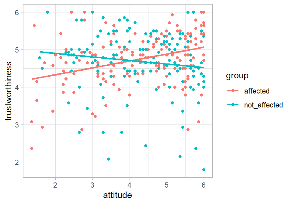

Figure 1.1: Trustworthiness vs. participant attitude to research

Exercise 4.2 Visual inspection of the scatterplot

Does the relationship between attitude and trustworthiness appear to be the same within each group?

Within the group that were told that the researcher was personally affected by their research:

The association between attitude and trustworthiness appears to be
A more positive attitude towards the research topic tends to be associated with values of trustworthiness.

Within the group that were told that the researcher was personally not_affected by their research:

The association between attitude and trustworthiness appears to be
A more positive attitude towards the research topic tends to be associated with values of trustworthiness.

The scatterplot can be improved through further customisation.

For example, to change the x- and y- labels, add the code:

+ xlab("Participants' attitude to the research")
+ ylab("Trustworthiness of researcher")

Feel free to customise the plot further if you feel it can be improved!

It is good practice to inspect the distributions of the data prior to analysis, for example, with geom_histogram() or geom_density(). We can check if the data appear normally distributed, or positively or negatively skewed. We can also check for outliers using geom_boxplot(). Get to know your data!

# look at the distribution of trustworthiness
trust_data %>% 
  ggplot(aes(trustworthiness)) +
  geom_histogram() 

# look at the distribution of attitude
trust_data %>% 
  ggplot(aes(attitude)) +
  geom_histogram() 

# obtain n in affected & not_affected groups
trust_data %>% 
  group_by(group) %>% 
  count()

4.5 Evidence for the interaction

An interaction between the attitude and group predictors is suggested by the scatterplot. That is, the association between trustworthiness and attitude appears to be different in the affected and non_affected groups. We may therefore want to include the interaction term in our multiple regression model and determine whether we have evidence for the interaction or not using Bayes factors.

We'll do this in three steps:

1. Specify the model without the interaction
1. Specify the model with the interaction
1. Compare the model with and without the interaction

4.5.1 Model without the interaction

The model without an interaction looks like a typical multiple regression model with two predictors (from Session 2):

model <- lm(outcome ~ predictor_1 + predictor_2, data = mydata)

As we did in the previous session, we need to also convert the categorical variable (group) to a factor() to ensure it's treated as categorical by R.

Thus, for our data:

# Convert group to a factor
trust_data <- trust_data %>% mutate(group = factor(group))

# Specify the model without the interaction
without_interaction <- lm(trustworthiness ~ attitude + group, 
                          data = trust_data)

# R² for the model
# load the broom package if you haven't already
# library(broom)
glance(without_interaction)

r.squared	adj.r.squared	sigma	statistic	p.value	df	logLik	AIC	BIC	deviance	df.residual	nobs
0.0130486	0.0065555	0.7588684	2.009602	0.1358188	2	-349.3972	706.7944	721.7018	175.0679	304	307

How much of the variance in trustworthiness is explained by the model with attitude and group? The adjusted R² (as a proportion, to two decimal places) = .

Did you know that R can round values to two decimal places for you?

Use this code in your script:

# round adjusted r-squared to 2.D.P
round(0.0065555, 2)

Next use lmBF() to obtain the BF for the model with no interaction:

# library(BayesFactor)

# obtain BF for the model
BF_without_interaction <- lmBF(trustworthiness ~ attitude + group,
                               data = data.frame(trust_data))

# look at the BF
BF_without_interaction

## Bayes factor analysis
## --------------
## [1] attitude + group : 0.102219 ±1.42%
## 
## Against denominator:
##   Intercept only 
## ---
## Bayes factor type: BFlinearModel, JZS

The BF for the model without the interaction is equal to (to 2 decimal places) .

You'll notice that the BF has ±4.03% or similar next to it in the output. This is the error associated with the BF. It's like saying my height is 185 cm, plus or minus 4 cm or so. It can be non-zero because generation of the BFs involves random sampling processes. Larger error values mean that the exact same value of the BF won't necessarily be output each time the line of code containing lmBF() is run, so there's a chance that the BFs in your output differ slightly from those above. It should be very low, and approximately 0.10 though.

4.5.2 Model with the interaction

To specify an interaction between two predictors, use the term predictor1 * predictor2. The * symbol means multiply, so the interaction term is simply the predictors multiplied together.

To specify the model with the interaction, add the interaction term predictor1 * predictor2 to the model without the interaction term:

# Specify the model with the interaction
with_interaction <- lm(trustworthiness ~ attitude + group + attitude*group,
                       data = trust_data)

# R² for the model
glance(with_interaction)

r.squared	adj.r.squared	sigma	statistic	p.value	df	logLik	AIC	BIC	deviance	df.residual	nobs
0.0623098	0.0530257	0.740907	6.711482	0.0002128	3	-341.5378	693.0756	711.7098	166.3298	303	307

How much of the variance in trustworthiness is explained by the model with attitude,group, and the attitude*group interaction? The adjusted R² (as a proportion, to two decimal places) = .

Use lmBF() to obtain the BF for the model with the interaction:

# obtain BF for the model
BF_with_interaction <- 
  lmBF(trustworthiness ~ attitude + group + attitude*group,
       data = data.frame(trust_data))

# look at the BF
BF_with_interaction

## Bayes factor analysis
## --------------
## [1] attitude + group + attitude * group : 31.04004 ±1.25%
## 
## Against denominator:
##   Intercept only 
## ---
## Bayes factor type: BFlinearModel, JZS

The BF for the model with the interaction is equal to . (Note: yours may come out slightly different to that shown in the worksheet due to random sampling processes used in the BF generation; as long as the BF is around 30, that's okay.)

4.5.3 Compare the model with and without the interaction

To determine whether there's evidence for the interaction, we need to compare the Bayes factor for the model with and without the interaction.

Exercise 4.3 Bayes factors can be compared with the formula:

\(\frac{Bayes \ factor \ more \ complex \ model}{Bayes \ factor \ simpler \ model}\)

Dividing the BFs in this way will return another Bayes factor, which is a number that tells us how many times more likely the more complex model compared to the simpler model, given the data.

So, if we perform this calculation:

\(\frac{Bayes \ factor \ for \ model \ with \ interaction}{Bayes \ factor \ for \ model \ without \ interaction}\)

this will tell us how many times more likely the model with the interaction is than the model without the interaction. In other words, dividing the BF for the model with the interaction by the BF for the model without the interaction will tell us whether there's evidence for an interaction between the predictors.

# compare BFs of models
# to determine evidence for the interaction
BF_with_interaction / BF_without_interaction

## Bayes factor analysis
## --------------
## [1] attitude + group + attitude * group : 303.6622 ±1.89%
## 
## Against denominator:
##   trustworthiness ~ attitude + group 
## ---
## Bayes factor type: BFlinearModel, JZS

The Bayes factor for the comparison of the model with and without the interaction is approximately 300. (Yours may not be exactly equal to 300 because of the error associated with the generation of the Bayes factor; it should be roughly the same though!)

Exercise 4.4 Assessing the interaction

Adjusted R²:

The adjusted R² for the model without the interaction (that you noted earlier) was:
The adjusted R² for the model with the interaction (that you also noted earlier) was:
What is the increase in adjusted R² as a result of the addition of the interaction term to the model? Hint. Work out the difference between the two adjusted R² values you noted above

Did you know that R can function like a calculator too? Simply type the formula next to > in the console window and hit enter, e.g., > 2 + 2

Or use code in your script:

# work out difference in R-squared
0.05 - 0.01

Bayes factors

According to comparison of BFs for the model with and without an interaction term included, which statement is true?

There's substantial evidence for an absence of an interaction between attitude and group The model with the interaction is as likely as the model without the interaction, given the data There's substantial evidence for an interaction between attitude and group

As a result of adding in the interaction term to the model, the adjusted R² value increases by approximately 0.04 (i.e., from 0.01 to 0.05). The comparison of BFs for the model with and without the interaction term indicates that there's substantial evidence for the interaction between attitude and group - it's around 300 times more likely that there is an interaction than there isn't one, given the data.

Thus, as indicated in the scatterplot, there's evidence that the association between trustworthiness and attitude is different in each group. Specifically, the association is positive in the affected group, whereas it appears to be negative in the not_affected group.

4.6 Simple slopes analysis

Given evidence for the interaction, we can conduct follow-up analyses to further characterise it.

In a simple slopes analysis the relationship between the outcome and first predictor is examined at each level of the second predictor.

Another way of thinking about the interaction is that it implies that the slopes of the lines for the affected group (red line in the scatterplot) and not_affected group (blue line) are not the same. We'll conduct a simple slopes analysis by conducting two simple regressions. The first will be the regression of trustworthiness on the basis of attitude in the affected group. The second will be the regression of trustworthiness on the basis of attitude in the not_affected group. The simplest way to do this is to store the data for each group separately, then perform a simple regression with each dataset.

First, filter trust_data for each group:

# Filter the dataset for when group is equal to "affected"
# store in affected_data
affected_data <- trust_data %>% filter(group == "affected")

# Filter the dataset for when group is equal to "not_affected"
# store in not_affected_data
not_affected_data <- trust_data %>% filter(group == "not_affected")

Now run a simple regression of trustworthiness ~ attitude in each group. First, do the affected group:

# affected group: simple regression coefficients
lm(trustworthiness ~ attitude, data = affected_data)

# affected group: BF
lmBF(trustworthiness ~ attitude, data = data.frame(affected_data))

## 
## Call:
## lm(formula = trustworthiness ~ attitude, data = affected_data)
## 
## Coefficients:
## (Intercept)     attitude  
##      3.9631       0.1839  
## 
## Bayes factor analysis
## --------------
## [1] attitude : 1483.223 ±0%
## 
## Against denominator:
##   Intercept only 
## ---
## Bayes factor type: BFlinearModel, JZS

Exercise 4.5 For the affected group (the red line in the scatter plot)

The intercept of the regression line is =
The slope of the regression line is =
The BF for the model (to two decimal places) is
This is evidence for association between trustworthiness and attitude in the affected group.
In this group, participants with more positive attitudes to the research topic perceived the researcher to be credible.

For the not_affected group:

# not_affected group: simple regression coefficients
lm(trustworthiness ~ attitude, data = not_affected_data)

# not_affected group BF
lmBF(trustworthiness ~ attitude, data = data.frame(not_affected_data))

## 
## Call:
## lm(formula = trustworthiness ~ attitude, data = not_affected_data)
## 
## Coefficients:
## (Intercept)     attitude  
##     5.09157     -0.09505  
## 
## Bayes factor analysis
## --------------
## [1] attitude : 0.5874073 ±0%
## 
## Against denominator:
##   Intercept only 
## ---
## Bayes factor type: BFlinearModel, JZS

Exercise 4.6 For the not_affected group (the blue line in the scatterplot)

The intercept of the regression line is =
The slope of the regression line is =
The BF for the model is
Although the scatterplot suggests association between trustworthiness and attitude in the not_affected group, there was insufficient evidence for this association because the Bayes factor was

In sum, this analysis has shown that when participants hold a more favourable attitude towards a research topic, they perceived researchers who were personally affected by their own research as being more trustworthy. Although the association appeared to be reversed for researchers who were not personally affected by their research, a Bayes factor analysis indicated that there was insufficient evidence of an association between trustworthiness and attitude in this group.

4.7 Exercises

Exercise 4.7 Credibility

In addition to asking about trustworthiness, Altenmuller et al. (2021) also asked participants how credible they found the researcher. The scores are stored in credibility in the trust_data; higher scores indicate greater perceived credibility. As with trustworthiness, the authors looked at whether attitude and group predicted credibility.

Adapt the code in this worksheet to do the following:

Create a scatterplot with credibility on the y-axis, attitude on the x-axis, and group as separate lines.

Pipe the data to ggplot() and use colour = group in aes

trust_data %>% 
  ggplot(aes(x = attitude, y = credibility, colour = group )) +
  geom_point() +
  geom_smooth(method = "lm", se = FALSE) +
  theme_light()

The slope for the affected group appears to be
The slope for the not_affected group appears to be

2. Obtain adjusted R² and the BF for the model without an interaction

Adjusted R² (as a proportion, to 2 decimal places) for the model without an interaction is:
The BF for the model without an interaction is

Specify the model with predictor1 + predictor2 with lm(), pass to glance(), then use lmBF() to get the BF.

# Specify the model without an interaction
credibility_no_interaction <- 
  lm(credibility ~ attitude + group, data = trust_data)

# library(broom)
glance(credibility_no_interaction)

# BF model
BF_credibility_no_interaction <-
  lmBF(credibility ~ attitude + group, data = data.frame(trust_data))

3. Obtain adjusted R² and the BF for the model with an interaction

Adjusted R² (as a proportion, to 2 decimal places) for the model with an interaction is:
The BF for the model with an interaction is x 10¹²

Specify the model with predictor1 + predictor2 + predictor1*predictor2 with lm(), pass to glance(), then use lmBF() to get the BF.

# Specify the model with an interaction
credibility_with_interaction <- 
  lm(credibility ~ attitude + group + attitude*group, data = trust_data)

# library(broom)
glance(credibility_with_interaction)

# BF model
BF_credibility_with_interaction <-
  lmBF(credibility ~ attitude + group + attitude*group, data = data.frame(trust_data))

It means a very large number! For more information see: FAQ (Opens a new tab.)

Please take care to notice "e+" or "e-" in the output for your Bayes factors. As you can see, BF₁₀ = 1.82 means something drastically different to BF₁₀ = 1.82 x 10²⁷, and you wouldn't want to make this kind of mistake when drawing statistical inferences!

4. Compare the models with and without the interaction

The increase in adjusted R² as a result of including the interaction term in the model is (as a proportion to 2 decimal places) =
The Bayes factor for the comparison of the models with and without the interaction =
Is there substantial evidence for an interaction between attitude and group in the prediction of percieved credibility of the researcher?

Work out the difference in adjusted R² in the model with and without the interaction.
Use BF_model_with_interaction / BF_model_without_interaction
If the BF > 3, then by convention we say there's substantial evidence for the interaction.

# Adj R-square difference
0.21 - 0.15

# Compare BFs
BF_credibility_with_interaction / BF_credibility_no_interaction

5. Simple slopes analysis

For the affected group:

The intercept of the regression line is =
The slope of the regression line is =
The BF for the model is x 10¹⁵
This is evidence for association between credibility and attitude in the affected group.
In this group, participants with more positive attitudes to the research topic perceived the researcher to credible.

For the not_affected group:

The intercept of the regression line is =
The slope of the regression line is =
The BF for the model is
This is evidence for association between credibility and attitude in the not_affected group.

Use filter() to separate out the groups of each dataset. Conduct one simple regression for the affected group. Conduct one simple regression for the not_affected group.

# Filter the dataset for when group is equal to "affected"
affected_data <- trust_data %>% filter(group == "affected")

# Filter the dataset for when group is equal to "not_affected"
not_affected_data <- trust_data %>% filter(group == "not_affected")

# affected group coefficients
lm(credibility ~ attitude, data = affected_data)

# affected group BF
lmBF(credibility ~ attitude, data = data.frame(affected_data))

# not_affected group coefficients
lm(credibility ~ attitude, data = not_affected_data)

# not_affected group BF
lmBF(credibility ~ attitude, data = data.frame(not_affected_data))

Exercise 4.8 Critical evaluation of the field

Altenmuller et al. (2021) also asked participants to report how critical they were in their evaluation of the entire research field. The scores are stored in evaluation in the trust_data; higher scores indicate that the participant evaluated the field more critically. As with the other outcome variables we've considered, the authors looked at whether attitude and group predicted evaluation.

Adapt the code in this worksheet to do the following:

Create a scatterplot with evaluation on the y-axis, attitude on the x-axis, and group as separate lines.

Pipe the data to ggplot() and use colour = group in aes()

trust_data %>% 
  ggplot(aes(x = attitude, y = evaluation, colour = group )) +
  geom_point() +
  geom_smooth(method = "lm", se = FALSE) +
  theme_light()

The slope for the affected group appears to be
The slope for the not_affected group appears to be

2. Obtain adjusted R² and the BF for the model without an interaction

Adjusted R² (as a proportion, to 2 decimal places) for the model without an interaction is:
The BF for the model without an interaction is x 10¹³

Specify the model with predictor1 + predictor2 with lm(), pass to glance(), then use lmBF() to get the BF.

# Specify the model without an interaction
evaluation_no_interaction <- 
  lm(evaluation ~ attitude + group, data = trust_data)

# library(broom)
glance(evaluation_no_interaction)

# BF model
BF_evaluation_no_interaction <-
  lmBF(evaluation ~ attitude + group, data = data.frame(trust_data))

3. Obtain adjusted R² and the BF for the model with an interaction

Adjusted R² (as a proportion, to 2 decimal places) for the model with an interaction is:
The BF for the model with an interaction is x 10¹⁸

Specify the model with predictor1 + predictor2 + predictor1*predictor2 with lm(), pass to glance(), then use lmBF() to get the BF.

# Specify the model with an interaction
evaluation_with_interaction <- 
  lm(evaluation ~ attitude + group + attitude*group, data = trust_data)

# library(broom)
glance(evaluation_with_interaction)

# BF model
BF_evaluation_with_interaction <-
  lmBF(evaluation ~ attitude + group + attitude*group, data = data.frame(trust_data))

4. Compare the model with and without the interaction

The increase in adjusted R² as a result of including the interaction in the model is (as a proportion to 2 decimal places) =
The Bayes factor for the model with the interaction vs. without =
Is there evidence for an interaction between attitude and group?

Work out the difference in adjusted R² in the model with and without the interaction.
Use BF_more_complex_model / BF_simpler_model
If the BF > 3, then there's substantial evidence for the interaction.

# Adj R-square difference
0.27 - 0.20

# Compare BFs
BF_evaluation_with_interaction / BF_evaluation_no_interaction

5. Simple slopes analysis

For the affected group:

The intercept of the regression line is =
The slope of the regression line is =
The BF for the model is x 10²⁰
This is evidence for association between evaluation and attitude in the affected group.
In this group, participants with more positive attitudes to the research topic evaluated the research field critically

For the not_affected group:

The intercept of the regression line is =
The slope of the regression line is =
The BF for the model is
This is evidence for an association between evaluation and attitude in the not_affected group.

Use filter() to separate out the groups of each dataset. Conduct one simple regression for the affected group. Conduct one simple regression for the not_affected group.

# Filter the dataset for when group is equal to "affected"
affected_data <- trust_data %>% filter(group == "affected")

# Filter the dataset for when group is equal to "not_affected"
not_affected_data <- trust_data %>% filter(group == "not_affected")

# affected group
lm(evaluation ~ attitude, data = affected_data)

# affected group BF
lmBF(evaluation ~ attitude, data = data.frame(affected_data))

# not_affected group
lm(evaluation ~ attitude, data = not_affected_data)

# not affected group BF
lmBF(evaluation ~ attitude, data = data.frame(not_affected_data))

4.8 Further exercise

Exercise 4.9 No interaction

Using the data from Teychenne and Hinkley (2016) that we used in Session 1, determine whether there is evidence for an interaction between anxiety_score and level of education in the prediction of screen_time. education is made up of groups 'No uni degree' and 'University degree'.

The data are located at:

https://raw.githubusercontent.com/chrisjberry/Teaching/master/1_mental_health_data.csv

The increase in adjusted R² associated with the addition of the interaction to the model is (as a proportion)
The Bayes factor comparing the model with and without the interaction is (to two decimal places)
There's substantial evidence that the relationship between anxiety_score and screen_time is in those who have a degree and those who don't.

Given the lack of evidence for an interaction, in an additive model containing only anxiety_score and education as predictors of screen_time:

Higher anxiety scores tended to be associated with hours of screen time, but the Bayes factor indicated that there was insufficient evidence for this association, BF = .
Individuals without a university degree tended to spend using screens (e.g., devices, TV, computer) each week than those with a university degree, BF =

# read the data to R using read_csv()
mentalh <- read_csv('https://raw.githubusercontent.com/chrisjberry/Teaching/master/1_mental_health_data.csv')

# scatterplot
mentalh %>% 
  ggplot(aes(x = anxiety_score, y = screen_time, colour = education )) +
  geom_point() +
  geom_smooth(method = "lm", se = FALSE) +
  theme_light() 

# Specify the model without an interaction
screen_time_no_interaction <- 
  lm(screen_time ~ anxiety_score + education, data = mentalh)

# in library(broom)
glance(screen_time_no_interaction) # adj R² = 0.06

# BF model
BF_screen_time_no_interaction <-
  lmBF(screen_time ~ anxiety_score + education, data = data.frame(mentalh))

# Specify the model with an interaction
screen_time_with_interaction <- 
  lm(screen_time ~ anxiety_score + education + anxiety_score*education, data = mentalh)

# library(broom)
glance(screen_time_with_interaction)  # adj R² = 0.06

# BF model
BF_screen_time_with_interaction <-
  lmBF(screen_time ~ anxiety_score + education + anxiety_score*education, data = data.frame(mentalh))

# Adj R-square difference
0.06 - 0.06

# Compare BFs
BF_screen_time_with_interaction / BF_screen_time_no_interaction

# There's no evidence for the interaction, 
# therefore assume additive model
#
# BF of unique contribution of anxiety_score in model with education
# This is the BF for model with both anxiety AND education,
# divided by the BF for the model where anxiety is left out
BF_screen_time_no_interaction / lmBF(screen_time ~ education, data = data.frame(mentalh))

# BF of unique contribution of education in model with anxiety_score
# This is the BF for model with both anxiety AND education,
# divided by the BF for the model where education is left out
BF_screen_time_no_interaction / lmBF(screen_time ~ anxiety_score, data = data.frame(mentalh))

It's possible to store R² values in variables. This can be handy if referring to them again in calculations, or if you want greater precision.

# Store adj r-sq for model with no interaction
rsq_no <- glance(screen_time_no_interaction)$adj.r.squared

# look at rsq
rsq_no


# Store adj r-sq for model with interaction
rsq_with <- glance(screen_time_with_interaction)$adj.r.squared

# look at rsq
rsq_with

# work out change in adj R^2^ as a result of adding the interaction 
rsq_with - rsq_no

Interestingly the change in adjusted R² is negative here. Remember that this is because the calculation of adjusted R² adjusts R² downwards, taking into account the additional predictor in the model. Performing the calculation with the non-adjusted R² values returns a (very small) positive number.

4.9 Further knowledge

4.9.1 Moderation

The analysis that we've performed with attitude and group in this session is sometimes referred to as a test of moderation (Baron & Kenny, 1986).

Moderation is when the relationship between two variables changes as a function of a third variable.

Altenmuller et al. (2021) concluded that participants' attitude moderated "the effect of a researcher disclosing being personally affected (vs. not affected ) by their own research on participants' trustworthiness ascriptions regarding the research". That is, attitude moderates the effect of group on trustworthiness.

It could also be said that the effect of a researcher saying that they are personally affected by their own research moderates the relationship between attitude and trustworthiness (or credibility). That is, the group moderates the relationship between attitude and trustworthiness. A relationship is present when the researcher says they are affected, but absent when they say they are not affected.

Which variable is said to be the moderator variable appears to be down to the choice of the researcher and the context of the research.

If we don't find evidence for the interaction term, then we don't have evidence that one variable moderates the relationship between the other two. Instead, researchers may say that there is an additive effect of both predictors on the outcome variable. The absence of an interaction indicates that the regression lines for each group do not differ (i.e., the lines for each group in a scatterplot are statistically parallel to one another).

4.9.2 Coefficients

Only for those wanting a deeper understanding.

If we obtain the coefficients for the full regression model (with the interaction), we can write out the regression equation:

lm(trustworthiness ~ attitude + group + attitude*group, data = trust_data)

\(Predicted\ outcome = a + b_1X_1 + b_2X_2 + b_3X_1X_2\)

So,

\(Predicted\ trustworthiness = 3.96 + 0.18(attitude) + 1.13(group) - 0.28(attitude\times group)\)

From this equation, we can derive the simple regression equations for each group.

As we saw in the previous session, behind the scenes, R uses dummy coding to code the two levels of the categorical variable (i.e., coding levels of a categorical variable with 0s and 1s). It uses 0s to code the affected group and 1s to code the not_affected group. It does it this way because it assigns 0s and 1s alphabetically.

Thus, taking the regression equation and substituting group = 0 for the affected group:

\[ \begin{align} Predicted\ trustworthiness &= 3.96 + 0.18(attitude) + (1.13\times0) - 0.28(attitude\times0)\\ &= 3.96 + 0.18(attitude) + 0 - 0 \\ &= 3.96 + 0.18(attitude) \end{align} \] The intercept (3.96) and slope (0.18) in this simple regression equation match those obtained for the affected group in the earlier simple slopes analysis.

Next, taking the full regression equation and substituting group = 1 for the not_affected group:

\[ \begin{align} Predicted\ trustworthiness &= 3.96 + 0.18(attitude) + (1.13\times1) - 0.28(attitude\times1)\\ &= 3.96 + 0.18(attitude) + 1.13 - 0.28(attitude) \\ &= 5.09 + 0.18(attitude) - 0.28(attitude) \\ &= 5.09 -0.10(attitude) \end{align} \]

The intercept (5.09) and slope (-0.10) in this simple regression correspond to those we obtained for the not_affected group in the earlier simple slopes analysis.

In sum, when one of the predictors is dichotomous, it is possible to derive the simple regression equation for each level of that predictor from the regression equation for the model with the interaction term included.

4.9.3 Centering

Again, only for those wanting deeper knowledge.

When testing for moderation effects, it is common to center the predictor variables prior to the analysis. (Indeed, Altenmuller et al. (2021) centered attitude prior to running their analyses.) Centering is where you subtract the mean of a variable from every score of that variable. For example, to center the attitude scores, we'd obtain the mean of attitude, and then subtract that value from each of our attitude scores. Thus, a participant with a score of 0 on the centered attitude score would therefore have an attitude value that is equal to the mean.

Centering is usually performed to help increase the interpretability of the coefficients of the predictor variables in a model with an interaction. It can also help to reduce the chances of multicollinearity between the predictor variables and the interaction term. Multicollinearity can occur because the interaction term is derived from the individual predictors themselves (by multiplying them together).

scale() can be used to center variables automatically. Set the option center = TRUE to center the variable. Setting the option scale = TRUE would also standardise the variable (i.e., divide each score by the standard deviation, to create z-scores), so scale = FALSE means that we won't also standardise the scores:

# center the attitude scores
# use mutate() to create a new variable in trust_data
# called attitude_centered
trust_data <- 
  trust_data %>% 
  mutate( attitude_centered = scale(attitude, center = TRUE, scale = FALSE)[,1] )

# compare the means to check that centered scores have mean of 0
trust_data %>% summarise(mean(attitude), mean(attitude_centered))

Before centering, the mean of the attitude scores was 4.26. After centering, the mean (of attitude_centered) is 0, or close enough to zero, being 4.08 x 10^-16, more precisely because there's some rounding error along the way.

Now re-run the analysis using attitude_centered in place of attitude and look at adjusted R² and the BF:

# full model with attitude_centered
full_centered <- lm(trustworthiness ~ attitude_centered + group + attitude_centered*group, data = trust_data)

# R-squared
glance(full_centered)

# BF
lmBF(trustworthiness ~ attitude_centered + group + attitude_centered*group, 
     data = data.frame(trust_data))

The adjusted R² for the full model is , which is the same as we found previously when attitude was not centered.
The BF for the model is approximately 33, which is the same as we found previously with the non-centered version of attitude.

Thus, centering predictors does not affect the adjusted R² or evidence for the model. This is because subtracting the mean from a variable is equivalent to a linear transformation and this does not affect the association.

To go even further, centering affects the values of the coefficients of the individual predictors in the model, but has no effect on the coefficient for the interaction.

When attitude wasn't centered, the regression equation was:

\(Predicted\ trustworthiness = 3.96 + 0.18(attitude) + 1.13(group) - 0.28(attitude\times group)\)

Using attitude_centered, the coefficients for the regression equation are obtained from:

full_centered

And so the regression equation is:

\(Predicted\ trustworthiness = 4.75 + 0.18(attitude) -0.06(group) - 0.28(attitude\times group)\)

Notice that the intercept has changed and so has the coefficient for group.

As before, to obtain the simple regression equations for each group we can once again substitute in the dummy codes for group. Thus, for the affected group:

\[ \begin{align} Predicted\ trustworthiness &= 4.75 + 0.18(attitude) - (0.06\times0) - 0.28(attitude\times0)\\ &= 4.75 + 0.18(attitude) + 0 - 0 \\ &= 4.75 + 0.18(attitude) \end{align} \]

For the not_affected group:

\[ \begin{align} Predicted\ trustworthiness &= 4.75 + 0.18(attitude) - (0.06\times1) - 0.28(attitude\times0)\\ &= 4.75 + 0.18(attitude) -0.06 - 0.28(attitude) \\ &= 4.69 + 0.18(attitude) - 0.28(attitude) \\ &= 4.69 -0.10(attitude) \end{align} \] The values in the simple regression equations come out slightly differently when attitude is centered, but the direction on the sign of the coefficient for attitude is the same.

In sum, centering of predictor variables is often performed in moderation analyses, but does not affect the variance explained by the model, nor the evidence (i.e., the BF) for the model, nor the direction (positive/negative) of the associations in the simple slopes analyses (because it doesn't change the slope). Centering can be desirable to aid interpretation of the coefficients of individual predictors and can reduce multicollinearity.

4.10 Summary

A multiple regression model can consist of a mixture of continuous and categorical predictors,
Predictors may have a combined effect in explaining the outcome variable. Evidence for this interaction effect can be examined by adding the interaction term to the model, i.e., with lm(outcome ~ predictor1 + predictor2 + predictor1*predictor2)
With a dichotomous categorical variable, the interaction implies that the slopes of the simple regressions of outcome ~ continuous_predictor are different. This can be examined with a simple slopes analysis.
The interaction implies that the relationship between the outcome and continuous predictor are different in each group.

4.11 References

Altenmuller M.S., Lange L.L., Gollwitzer M. (2021). When research is me-search: How researchers’ motivation to pursue a topic affects laypeople’s trust in science. PLoS ONE 16(7): e0253911. https://doi.org/10.1371/journal.pone.0253911

Baron, R. M., & Kenny, D. A. (1986). The moderator–mediator variable distinction in social psychological research: Conceptual, strategic, and statistical considerations. Journal of Personality and Social Psychology, 51(6), 1173. https://psycnet.apa.org/doi/10.1037/0022-3514.51.6.1173