Session 7 Pre-post data, clinically significant change
Chris Berry
2026
7.1 Overview
- Slides for the lecture accompanying this worksheet are on the DLE.
- R Studio online Access here using University log-in
To investigate the effect of an intervention, researchers may measure a dependent variable before and after the intervention. For example, a researcher might look at the impact of a particular treatment (or therapy) on the severity of depression symptoms. The data produced is sometimes referred to as pre-post data.
Pre-post data in the treatment group is often compared with that of a control group.
There are numerous ways to analyse the data from such designs. Three approaches are presented here, alongside an introduction to methods for calculating clinically significant change.
7.1.1 Worked example
Francis et al. (2019) investigated whether a shift to a healthy diet impacted on depression in a group of individuals that had diets that fell short of the criteria for healthy eating, as defined by the Australian Guide to Healthy Eating. There were 76 participants. All had moderate to severe symptoms of depression.
Half of the participants received instruction on guidance regarding their diet. Severity of depression symptoms were measured at two time points: before the intervention, and again three weeks later.
Exercise 7.1 Design Check
What is the name of the first independent variable mentioned?
Is the first independent variable manipulated between- or within-subjects?
How many levels does the first independent variable have?
What is the name of the second independent variable mentioned in the study?
Is the second independent variable manipulated between- or within-subjects?
How many levels does the second independent variable have?
What is the dependent variable?
7.1.2 Read in the data
# read in
diet <- read_csv('https://raw.githubusercontent.com/chrisjberry/Teaching/master/7_diet_depression.csv')

# preview
diet %>% head()| ppt | group | baseline | week3 |
|---|---|---|---|
| 1 | diet_change | 18.00000 | 11.00000 |
| 2 | diet_change | 34.00000 | 11.00000 |
| 3 | diet_change | 28.42105 | 3.00000 |
| 4 | diet_change | 25.00000 | 14.00000 |
| 5 | diet_change | 40.00000 | 49.00000 |
| 6 | diet_change | 15.00000 | 14.73684 |
Exercise 7.2 Data Check
How many participants are there in
diet?Are the data in
dietin long format or wide format?
Each participant's data is on a separate row. There is a column to code the group membership. The scores for each time condition, baseline and week3, are in separate columns. Therefore the data are in wide format. You can inspect all the data in a separate data viewer with the code View(diet). (Note that although there are 76 participants on 76 rows, the ppt identifiers go up to 77; this is because the data for participant 50 were incomplete and were therefore excluded.)
- What do the scores in the
baselineandweek3columns represent?
7.1.3 Plot the means
To plot the means, we need the data to be in long format:
# The code below:
# - stores the result in diet_long
# - takes diet and pipes it to
# - pivot_longer()
# - specifies which of the existing columns to make into a single new column ('cols')
# - specifies the name of the new column labeling the conditions ('names_to')
# - specifies the name of the column containing the dependent variable ('values_to')
diet_long <-
  diet %>%
  pivot_longer(cols = c(baseline, week3),
               names_to = "time",
               values_to = "symptoms")

# preview
diet_long %>% head()| ppt | group | time | symptoms |
|---|---|---|---|
| 1 | diet_change | baseline | 18.00000 |
| 1 | diet_change | week3 | 11.00000 |
| 2 | diet_change | baseline | 34.00000 |
| 2 | diet_change | week3 | 11.00000 |
| 3 | diet_change | baseline | 28.42105 |
| 3 | diet_change | week3 | 3.00000 |
Now use diet_long with ggdotplot() in the ggpubr package.
library(ggpubr)

diet_long %>%
  ggdotplot(x = "time",
            y = "symptoms",
            color = "group",
            add = "mean_se",
            ylim = c(0,65),
position_dodge = 0.1) 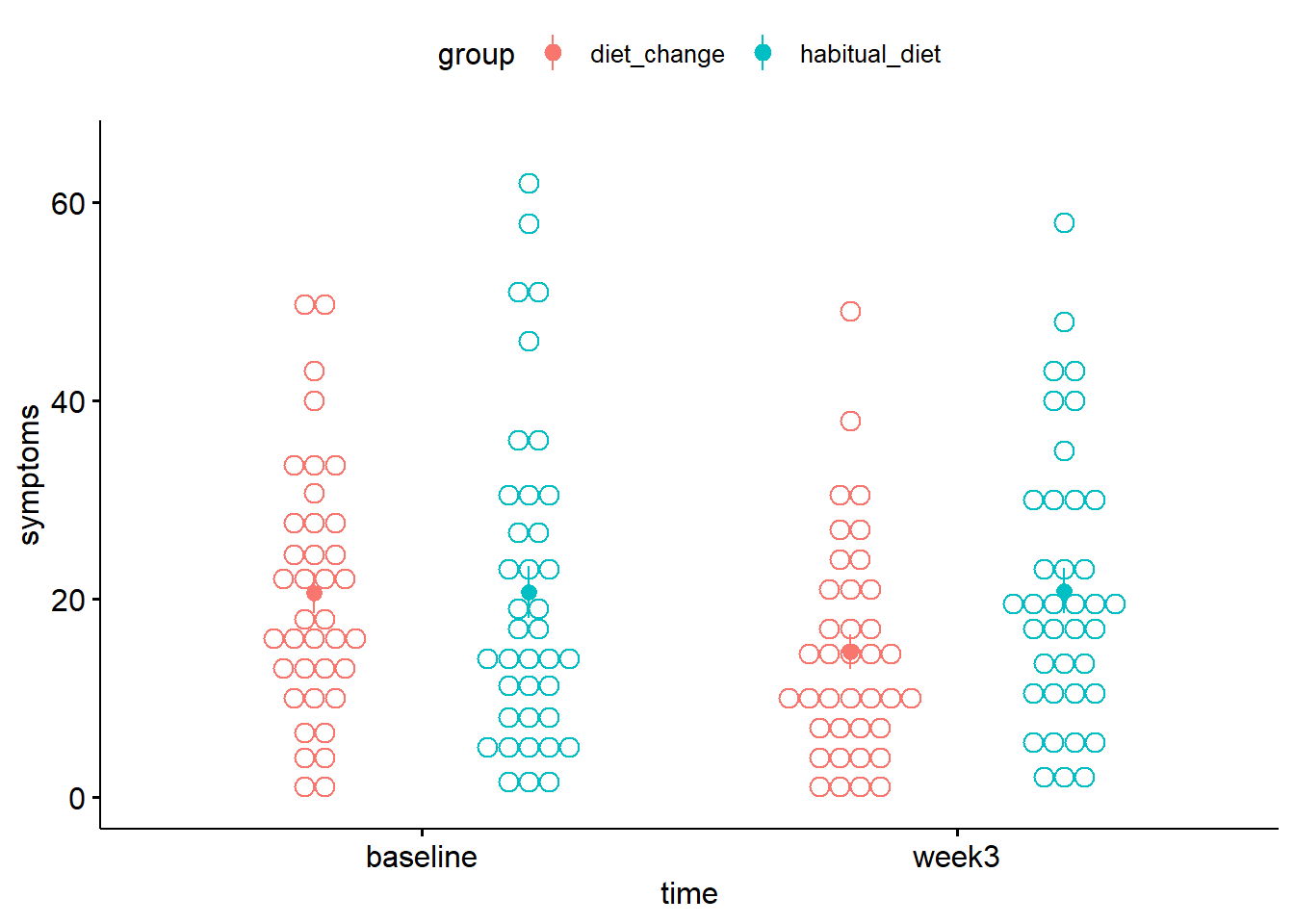
Figure 2.1: Mean depression symptoms score. Solid circles denote the mean, error bars the SE.
Each dot represents one participant's data. The solid circles indicate the mean severity of depression symptoms in each condition (with between-subject error bars added by using add = mean_se). (See Session 6 for further details on producing within-subject error bars, which may be more appropriate here.) Higher scores indicate greater severity.
- In the
diet_changegroup, from baseline to week 3, the mean severity of symptoms appeared to . - In the
habitual_dietgroup, from baseline to week 3, the mean severity of symptoms appeared to .
7.2 Approach 1 - Difference scores
One approach to analysing pre-post data is to compare the change in symptom scores from baseline to week3 across groups. This is achieved by 1) calculating the difference in scores between baseline and week3, and then 2) comparing the difference scores between the two groups using a between-subjects ANOVA (or, equivalently, a t-test).
To calculate the change in severity score for each participant, it's simplest to use the wide format data since we can easily subtract scores in one column (week3) from another (baseline).
# using the wide format data
# calculate the difference in baseline and week3 scores
# store in a new column called 'change'
diet <-
  diet %>%
  mutate(change = week3 - baseline)

# look at new column
diet %>% head()| ppt | group | baseline | week3 | change |
|---|---|---|---|---|
| 1 | diet_change | 18.00000 | 11.00000 | -7.0000000 |
| 2 | diet_change | 34.00000 | 11.00000 | -23.0000000 |
| 3 | diet_change | 28.42105 | 3.00000 | -25.4210526 |
| 4 | diet_change | 25.00000 | 14.00000 | -11.0000000 |
| 5 | diet_change | 40.00000 | 49.00000 | 9.0000000 |
| 6 | diet_change | 15.00000 | 14.73684 | -0.2631579 |
The column change now contains the change in symptom severity score from baseline to week3. A negative difference indicates an improvement in symptoms (i.e., the score at week3 was lower).
To compare the change scores between the two groups, use anovaBF(). The functions lmBF() or ttestBF() could also be used. They all give equivalent results because there are only two groups being compared.
# Convert the grouping variable 'group' to a factor
diet <-
  diet %>%
  mutate(group = factor(group))

# anovaBF(): between-subjects ANOVA
anovaBF(change ~ group, data = data.frame(diet))
## Bayes factor analysis
## --------------
## [1] group : 2.262527 ±0.01%
##
## Against denominator:
## Intercept only
## ---
## Bayes factor type: BFlinearModel, JZS# lmBF(): between-subjects ANOVA
lmBF(change ~ group, data = data.frame(diet))
# ttestBF: between-subjects
ttestBF(x = diet$change[ diet$group == "habitual_diet" ],
y = diet$change[ diet$group == "diet_change" ]) ## Bayes factor analysis
## --------------
## [1] group : 2.262527 ±0.01%
##
## Against denominator:
## Intercept only
## ---
## Bayes factor type: BFlinearModel, JZS
##
## Bayes factor analysis
## --------------
## [1] Alt., r=0.707 : 2.262527 ±0.01%
##
## Against denominator:
## Null, mu1-mu2 = 0
## ---
## Bayes factor type: BFindepSample, JZS- The Bayes factor comparing the change in severity of depression symptoms between baseline and week 3 is (to two decimal places) .
- Although there is evidence for a difference in the change score between groups, the Bayes factor was .
- Thus, by the method of comparing change scores between groups, can we conclude that the dietary intervention led to a reduction in depression symptom severity?
7.3 Approach 2 - Mixed ANOVA
Given that we have two independent variables, each with two levels, and where one is manipulated between-subjects and the other within-subjects, it is also possible to treat the design as a 2 x 2 mixed factorial design and analyse the data using anovaBF().
Because one of the factors is manipulated within-subjects, we need to add ppt to the model and specify it as a random factor using whichRandom = "ppt" (see Session 6). We also need to convert ppt to a factor, along with the other independent variables, group and time.
As with repeated measures ANOVA in Session 6, the long format data needs to be used for the analysis.
# convert ppt and IVs to factors
diet_long <-
  diet_long %>%
  mutate(ppt   = factor(ppt),
         group = factor(group),
         time  = factor(time))

# anova model
bfs <- anovaBF(symptoms ~ group + time + ppt, whichRandom = "ppt", data = data.frame(diet_long))

# look at the bfs
bfs
In this analysis, we are less interested in the main effects of group and time and are more interested in the interaction between the factors. The interaction will tell us whether the change in symptom severity differs between groups. As with previous two-way ANOVAs, the BF for the interaction can be obtained by dividing the BF in [4] by the BF in [3] (see Sessions 3 and 6).
- The Bayes factor representing evidence for the interaction term is .
The Bayes factor for the interaction should come out at around 2.25, but because anovaBF() calculates the BF using random sampling methods, your value may not match this exactly (note the large error associated with the BF in the output). For greater precision, it's possible to recompute() the Bayes factor with a greater number of random samples, e.g., 1,000,000 (note, this could take a short while):
# recompute bfs, but with a million iterations
bfs_more <- recompute(bfs, 1000000)

# re-obtain the BF for the interaction, using bf_more
bfs_more[4] / bfs_more[3]- The Bayes factor for the interaction, using
bf_moreis . - Although there is evidence for a difference in the change score between groups, the Bayes factor was .
- As a result of using a mixed ANOVA, can we conclude that the dietary intervention led to a reduction in depression symptom severity?
7.4 Approach 3 - ANCOVA
A third approach to analysing pre-post data is to use ANCOVA, which stands for Analysis of COvariance. This approach is particularly appropriate if our focus were solely on comparing the scores at the second time point between groups, but controlling for baseline symptom severity.
A covariate is a background variable that may be associated with the outcome variable, but is not of primary interest. In ANCOVA, the variance explained by a covariate is first accounted for, before examining whether the dependent variable differs between groups or conditions. Because some of the error variance is explained by the covariate, ANCOVAs can have the advantage of being more powerful tests of the predictor of interest.
The ANCOVA is essentially a one-way between subjects ANOVA, with symptom severity at week3 as the dependent variable, group as the independent variable, and symptoms at baseline as the covariate.
Equivalently, the analysis can be conceptualised is a multiple regression of week3 scores on the basis of group and baseline. Assessing the unique contribution of group will tell us whether there's a difference in symptom severity at week3, after accounting for the variance explained by baseline scores (see Sessions 2 and 4)).
Note that because effects of time are not analysed in this approach, there is no repeated measures factor, and ppt does not need to be included as a random factor.
# The model with both group and baseline scores
full <- lmBF(week3 ~ group + baseline, data = data.frame(diet))

# The model with baseline scores only (for comparison)
baseline <- lmBF(week3 ~ baseline, data = data.frame(diet))

# The BF representing evidence for the unique contribution of group
full / baseline
## Bayes factor analysis
## --------------
## [1] group + baseline : 6.124479 ±0.83%
##
## Against denominator:
## week3 ~ baseline
## ---
## Bayes factor type: BFlinearModel, JZS- The Bayes factor for the unique contribution of
groupis . - There is evidence for a difference in the
week3scores between groups, after controlling forbaselinescores. - As a result of using the ANCOVA approach, can we conclude that the dietary intervention led to a reduction in depression symptom severity?
In Approach 3 R2 for the effect of group can be determined using methods from earlier sessions. The method is equivalent to obtaining R2 for the unique contribution of a predictor.
# ensure broom is loaded
# library(broom)

# specify the full model with lm()
full_model    <- lm(week3 ~ group + baseline, data = diet)

# specify the model with baseline only
baseline_only <- lm(week3 ~ baseline, data = diet)

# R-squared full model
glance(full_model)$r.squared

# R-squared baseline only
glance(baseline_only)$r.squared

# Unique contribution of group
# (effect size associated with difference in groups)
glance(full_model)$r.squared - glance(baseline_only)$r.squared # R-sq = 0.05817
7.5 Which approach should you use?
Which method you use depends on the research question you are asking.
If your question is whether the change in the dependent variable across timepoints differs between the two groups, then Methods 1 or 2 are appropriate.
If your question is whether one group has a higher mean at the second timepoint, then Method 3 seems most appropriate. Indeed, ANCOVA is often recommended for pre-post designs (see e.g., O'Connel et al., 2017). An advantage of the ANCOVA method is that is has greater statistical power. It is the approach that Francis et al. (2019) used.
7.6 Clinical Significance
The measure of depressive symptoms used by Francis et al. (2019) was the Centre for Epidemiological Studies Depression scale-Revised (CESD-R; Radloff, 1977). The scale ranges from 0-60, and the criterion for being the elevated range of depressive symptoms is a score equal to 16 or above.
Re-plot the data, but with a horizontal line to indicate this criterion.
diet_long %>%
  ggdotplot(x = "time",
            y = "symptoms",
            color = "group",
            add = "mean_se",
            ylim = c(0,65),
            position_dodge = 0.1) +
  geom_hline(yintercept = 16, colour = "red", lty = 2)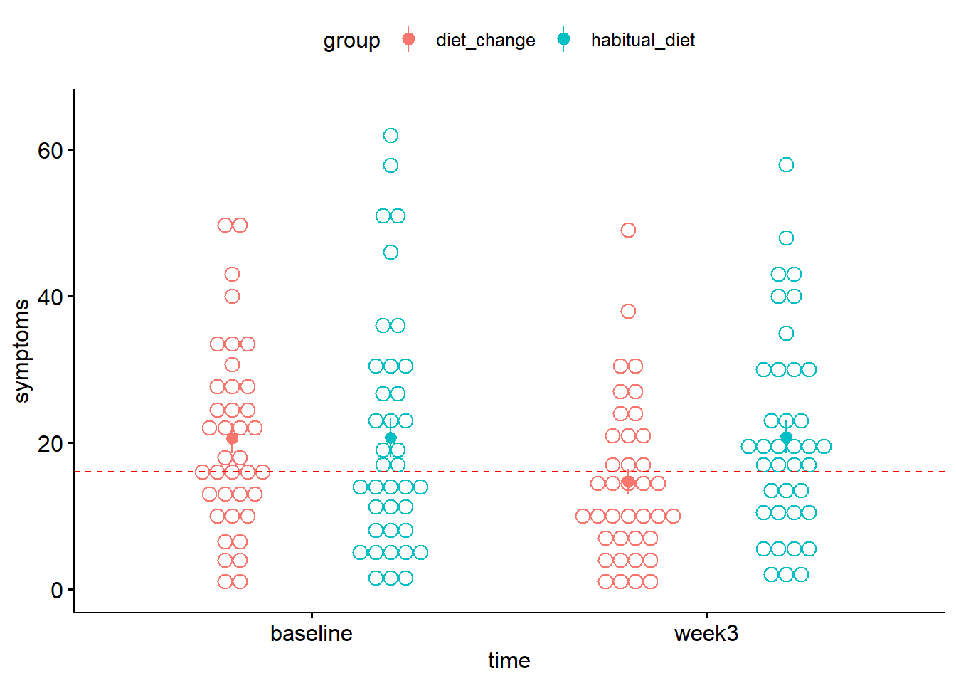
Figure 7.1: Mean depression symptom severity score in each condition. The dotted line indicates the criterion for the elevated range of depressive symptoms
- At baseline, was the mean of the
diet_changegroup above or below the criterion for clinical significance in the severity of depression symptoms? - After 3 weeks, was the mean of the
diet_changeabove or below the criterion for clinical significance in the severity of depression symptoms?
Note that these statements apply to the conditions as a whole, rather than the individuals in each condition. For instance, there may be individuals whose symptoms did not improve. To learn more about whether a given individual can be said to have improved or not, see the Further Knowledge section below.
7.7 Exercises
Exercise 7.3 Pre-post self-efficacy scores
Francis et al. (2019) also measured self-efficacy before and after the dietary intervention. Self-efficacy refers to a person's belief in their ability to exert control over their behaviours and circumstances they find themselves in. Higher scores indicate greater levels of self-efficacy.
Read in the data at the link below to self_efficacy and answer the questions.
https://raw.githubusercontent.com/chrisjberry/Teaching/master/7_diet_self_efficacy.csv
1. Create a plot of the mean self-efficacy before and after the intervention in each group
- Read the data using
read_csv() - Convert to long format
- Use a suitable package to plot the data. For example,
ggdotplot()in theggpubrpackage.
# read in
self_efficacy <- read_csv('https://raw.githubusercontent.com/chrisjberry/Teaching/master/7_diet_self_efficacy.csv')

# convert to long format
self_efficacy_long <-
  self_efficacy %>%
  pivot_longer(cols = c("baseline", "week3"),
               names_to = "time",
               values_to = "score")

# plot
self_efficacy_long %>%
  ggdotplot(x = "time", y = "score", color = "group", add = "mean_se",
            ylab = "Self-efficacy score")
2. Evidence for the dietary intervention on self-efficacy
- Using Approach 1, determine the Bayes factor representing the evidence for a difference in the change in self-efficacy score between the
diet_changeandhabitual_dietgroups. BF = - Using Approach 2, determine the Bayes factor, representing the evidence for a difference in the change in self-efficacy score score between groups. BF =
- Using Approach 3, determine the Bayes factor, representing the evidence for a difference in self-efficacy scores between groups at week 3, after controlling for self-efficacy scores at baseline. BF =
Is there substantial evidence for an effect of the dietary intervention on self-efficacy scores according to any of the approaches?
- Approach 1: ANOVA of difference scores.
- Approach 2: Mixed ANOVA.
- Approach 3: ANCOVA.
- Use the data in wide format.
- Create a column of difference scores using
mutate() - Compare the difference scores between groups using
anovaBF()(orlmBF()orttestBF()).
- Convert the data to long format using
pivot_longer(). - Convert the columns labelling the participant and independent variables to factors using
factor(). - Use
anovaBF()to run the 2 x 2 ANOVA, with the participant column as a random factor. - Obtain the Bayes factor for the interaction.
- Use the data in wide format.
- Use
lmBF()with the scores atweek3as the outcome variable andgroupandbaselineas predictors. - Use
lmBF()with the scores atweek3as the outcome variable andbaselineas the predictor. - Divide the BF for the model with both
groupandbaselineby the BF for the model withbaselinealone in order to determine the evidence that the scores atweek3differ betweengroupafter controlling forbaseline.
# Approach 1 - difference
self_efficacy <-
  self_efficacy %>%
  mutate(change = week3 - baseline,
         group = factor(group))

# using anovaBF
anovaBF(change ~ group, data = data.frame(self_efficacy))

# or lmBF
lmBF(change ~ group, data = data.frame(self_efficacy))

# or ttest
ttestBF(self_efficacy$change[self_efficacy$group=="habitual_diet"],
self_efficacy$change[self_efficacy$group=="diet_change"]) # Approach 2 - Mixed ANOVA
# set factors
self_efficacy_long <-
self_efficacy_long %>%
mutate(time = factor(time),
ppt = factor(ppt),
group = factor(group))
# get bfs
BFs <- anovaBF(score ~ group + time + ppt, whichRandom = "ppt", data = data.frame(self_efficacy_long))
BFs[4] / BFs[3]
# recompute
BFs2 <- recompute(BFs, 1000000)
BFs2[4] / BFs2[3] # Approach 3 - ANCOVA
# wide format
# convert to factors
self_efficacy <-
self_efficacy %>%
mutate(group = factor(group))
# specify group + baseline
BF_group_baseline <- lmBF(week3 ~ group + baseline, data = data.frame(self_efficacy))
# specify baseline only
BF_baseline <- lmBF(week3 ~ baseline, data = data.frame(self_efficacy))
# unique contribution group
BF_group_baseline / BF_baseline
7.8 Further Knowledge
7.8.1 Reliable Change (RC) index
In the main part of the worksheet, the mean symptom severity in the dietary intervention group moved from being above the criterion for the elevated range before the intervention to being below the criterion afterwards.
One way to determine whether a particular individual shows a clinically significant change involves calculating a Reliable Change (RC) index (Christensen & Mendoza, 1986; Jacobson & Trurax, 1991). The RC index can be calculated for each individual as follows:
\(RC = \frac{X_1 - X_2}{SE_D}\)
where \(X_1\) is an individual's pretest score, \(X_2\) is the posttest score, and \(SE_D\) is the standard error of the difference scores.
\(SE_D\) is calculated with the equation:
\(\sqrt{2(SD_{Pre}\sqrt{(1-\alpha)})^2}\)
where \(SD_{pre}\) is the standard deviation of the pre-test scores and \(\alpha\) is the reliability of the measure (e.g., Cronbach's alpha).
\(\alpha\) is necessary for the calculation of \(SE_D\), but was not reported by Francis et al. (2019). The CESD-R scale is widely used though, and Busch et al. (2011) derived an estimate of \(SE_D\) to be 5.05, using an \(\alpha\) of .914 and \(SD_{Pre}\) score of 12.187. For the purposes of illustration, we'll assume the value of \(SE_D\) is the same as in Busch et al. (2011) (i.e., 5.05).
If RC > 1.96 (or RC < -1.96, depending on the way the difference is calculated), then the individual can be said to show a reliable change.
Thus, to calculate RC for each individual in the diet_change group:
# filter the data for the diet_change group only
diet_change <-
  diet %>% filter(group == "diet_change")

# SE of differences
se_diff <- 5.05 # from Busch et al. (2011)

# Reliable Change index calculation
diet_change <-
  diet_change %>%
  mutate(RC = change / se_diff)

# preview
diet_change %>% head()| ppt | group | baseline | week3 | change | RC |
|---|---|---|---|---|---|
| 1 | diet_change | 18.00000 | 11.00000 | -7.0000000 | -1.3861386 |
| 2 | diet_change | 34.00000 | 11.00000 | -23.0000000 | -4.5544554 |
| 3 | diet_change | 28.42105 | 3.00000 | -25.4210526 | -5.0338718 |
| 4 | diet_change | 25.00000 | 14.00000 | -11.0000000 | -2.1782178 |
| 5 | diet_change | 40.00000 | 49.00000 | 9.0000000 | 1.7821782 |
| 6 | diet_change | 15.00000 | 14.73684 | -0.2631579 | -0.0521105 |
RC scores less than -1.96 indicate that the individual's score showed a reliable improvement in depressive symptoms (i.e., reliably lower scores on the CESD-R).
To see all the individuals who showed such a reduction:
| ppt | group | baseline | week3 | change | RC |
|---|---|---|---|---|---|
| 2 | diet_change | 34.00000 | 11 | -23.00000 | -4.554455 |
| 3 | diet_change | 28.42105 | 3 | -25.42105 | -5.033872 |
| 4 | diet_change | 25.00000 | 14 | -11.00000 | -2.178218 |
| 8 | diet_change | 33.00000 | 9 | -24.00000 | -4.752475 |
| 23 | diet_change | 43.00000 | 30 | -13.00000 | -2.574257 |
| 28 | diet_change | 22.00000 | 8 | -14.00000 | -2.772277 |
| 33 | diet_change | 50.52632 | 23 | -27.52632 | -5.450756 |
| 34 | diet_change | 28.00000 | 17 | -11.00000 | -2.178218 |
| 36 | diet_change | 49.00000 | 14 | -35.00000 | -6.930693 |
| 37 | diet_change | 23.00000 | 10 | -13.00000 | -2.574257 |
7.8.1.1 Scatterplot with RC bounds
All the data can be represented on a plot with bounds for reliable change as follows:
diet_change %>%
  ggplot(aes(x = baseline, y = week3)) +
  geom_point() +
  geom_abline() +
  geom_abline(slope = 1, intercept = -1.96*se_diff, lty = 2) +
geom_abline(slope = 1, intercept = 1.96*se_diff, lty = 2) 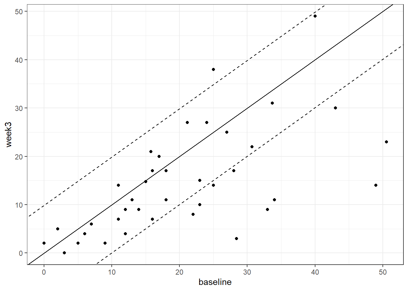
Figure 3.4: Baseline vs. week 3 depressive symptom severity in the diet change group. Dotted lines denoted Reliable Change index bounds
The black dashed lines are those plotted with geom_abline() and are created by multiplying se_diff by +1.96 and -1.96.
The points falling above the upper black dashed line indicate participants showing reliable worsening of depressive symptoms at the posttest compared to the the pretest.
The points falling below the lower black dashed line are individuals showing a reliable improvement (i.e., fewer depressive symptoms) at the posttest.
Francis et al. (2019) reported that 10 individuals showed a reliable improvement in the diet change group, as indicated by their RC scores. Only 4 individuals in the habitual diet group were reported to show a reliable improvement.
Count how many individuals fall below the lower black dashed line on the scatterplot, and can therefore be considered to meet the criteria for showing reliable improvement, as defined by the RC index?
The same process could be followed for the habitual_diet group to compare the number of individuals showing reliable change according to the RC index between groups. The code for this group is below. With the value of se_diff we've used here, a fifth person in this group has an RC index (just) exceeding -1.96. There's still half as many participants showing a reliable change, compared to the diet_change group.
The results obtained with RC index converge with those of the ANCOVA, and support the notion that a healthy diet can lead to improvement in the severity of depression symptoms.
# filter the data for the habitual_diet group only
habitual_diet <-
  diet %>% filter(group == "habitual_diet")

# SE of differences
se_diff <- 5.05 # from Busch et al. (2011)

# Reliable Change index calculation
habitual_diet <-
  habitual_diet %>%
  mutate(RC = change / se_diff)

# RC plot
habitual_diet %>%
  ggplot(aes(x = baseline, y = week3)) +
  geom_point() +
  geom_abline() +
  geom_abline(slope = 1, intercept = -1.96*se_diff, lty = 2) +
geom_abline(slope = 1, intercept = 1.96*se_diff, lty = 2) 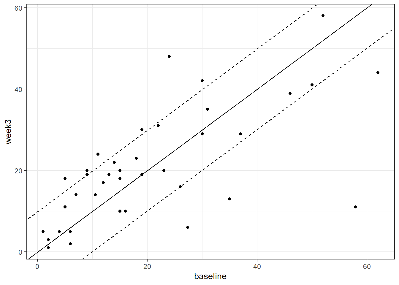
Figure 3.5: Baseline vs. week 3 depressive symptom severity in the habitual diet group. Dotted lines denoted Reliable Change index bounds
7.9 Summary
There are three main approaches for measuring pre-post data when there is a treatment and control group:
- Analysis of the difference scores in a between-subjects ANOVA.
- A 2 x 2 mixed ANOVA, with time (pre, post) as the within-subjects factor, and group (treatment, control) as the between-subjects factor.
- An ANCOVA comparing posttest scores between groups, after accounting for pretest scores as a covariate. This is equivalent to a multiple regression of posttest scores on the basis of pretest scores and group (i.e., one continuous and one categorical predictor).
- A result can be statistically significant, but not necessarily clinically significant. Various methods exist for establishing clinical significance, including using established scale cutoffs and using the Reliable Change Index.
7.10 References
Busch, A. M., Wagener, T. L., Gregor, K. L., Ring, K. T., & Borrelli, B. (2011). Utilizing reliable and clinically significant change criteria to assess for the development of depression during smoking cessation treatment: The importance of tracking idiographic change. Addictive Behaviors, 36(12), 1228-1232.
Christensen, L. & Mendoza, J. L. (1986). A method of assessing change in a single subject: an alteration of the RC index. Behavior Therapy. 17, 305-308.
Francis H.M., Stevenson R.J., Chambers J.R., Gupta D., Newey B., Lim C.K. (2019) A brief diet intervention can reduce symptoms of depression in young adults – A randomised controlled trial. PLoS ONE, 14(10): e0222768. https://doi.org/10.1371/journal.pone.0222768
Jacobson, N. S., & Truax, P. (1991). Clinical significance: A statistical approach to defining meaningful change in psychotherapy research. Journal of Consulting and Clinical Psychology, 59(1), 12–19. https://doi.org/10.1037/0022-006X.59.1.12
O'Connell, N. S., Dai, L., Jiang, Y., Speiser, J. L., Ward, R., Wei, W., ... & Gebregziabher, M. (2017). Methods for analysis of pre-post data in clinical research: a comparison of five common methods. Journal of Biometrics & Biostatistics, 8(1), 1. https://doi.org/10.4172/2155-6180.1000334
Radloff, L. S. (1977). The CES-D scale: A self-report depression scale for research in the general population. Applied Psychological Measurement, 1(3), 385-401.